Code Coverage Tools : In this comprehensive and beginner-friendly tutorial, we will explore the world of code coverage tools, which play a crucial role in ensuring your software is thoroughly tested and reliable. Whether you’re working on embedded systems, desktop applications, or large-scale software projects, understanding code coverage is essential for improving software quality and identifying untested parts of your codebase.
By the end of this tutorial, you will have a solid understanding of how code coverage tools work and how to integrate them into your own development workflow. Whether you are a student, a developer in testing, or an embedded systems engineer, this guide will empower you to write better-tested and more robust code in 2025 and beyond.
What Is Code Coverage?
Code coverage is a metric used to measure how much of your source code has been executed (or “covered”) during testing. It helps answer questions like:
Have all functions been tested?
Have all branches or conditions been exercised?
Are there any unused lines of code?
In simple terms, code coverage tools help ensure your tests are doing their job.
Why Code Coverage Matters
✅ Identifies untested parts of code
🚨 Helps find dead code or redundant logic
🔍 Improves software reliability
📊 Provides quality insights for QA, DevOps, and Developers
💬 Useful in code reviews and CI/CD pipelines
Types of Code Coverage Metrics
Type
Description
Example
Line Coverage
% of lines executed
90 out of 100 lines = 90%
Function Coverage
% of functions called
8 of 10 functions = 80%
Branch Coverage
% of if/else branches executed
Both if and else parts
Condition Coverage
% of boolean sub-expressions tested
if (A && B) tests A and B
Path Coverage
% of possible execution paths tested
All loops + conditions
Popular Code Coverage Tools
Tool
Language
Platform
Usage
gcov
C/C++
Linux
Built-in with GCC
lcov
C/C++
Linux
Visual frontend for gcov
gcovr
C/C++
Cross-platform
Outputs XML/HTML
JaCoCo
Java
Cross-platform
Java code coverage
Coverage.py
Python
Cross-platform
Simple and powerful
Istanbul
JavaScript
Node.js
For JS/TS projects
Tutorial: Using gcov and lcov (For C/C++ Beginners)
This tool summarizes all .gcov into HTML – very handy!
Summary
Code coverage tools help validate testing effectiveness.
For C/C++, gcov, lcov, and gcovr are most used.
Compile with coverage flags, execute the binary, then generate reports.
Visual tools help QA, CI, and reviews.
Code coverage != code quality but is a crucial metric.
We’ll:
Write a simple C program.
Compile it with code coverage flags.
Run it to generate coverage data.
Use gcov to view the coverage.
Optionally, use lcov + genhtml to generate an HTML report.
Step-by-Step Code Coverage Example with Code
Step 1: Write the C Program (math_utils.c)
// math_utils.c
#include <stdio.h>

int add(int a, int b) {
    return a + b;
}

int subtract(int a, int b) {
    return a - b;
}

int multiply(int a, int b) {
    return a * b;
}

int divide(int a, int b) {
    if (b == 0) {
        printf("Division by zero error!\n");
        return 0;
    }
    return a / b;
}

int main() {
    printf("Add: %d\n", add(5, 3));
    printf("Subtract: %d\n", subtract(5, 3));
    // multiply and divide not called

    return 0;
}
This creates extra files like math_utils.gcno (for structure data).
Step 3: Run the Program
./math_utils
Output:
Add: 8
Subtract: 2
This execution will generate math_utils.gcda (runtime data file showing which lines ran).
Step 4: Run gcov to See Coverage
gcov math_utils.c
You’ll see something like:
File 'math_utils.c'
Lines executed:60.00% of 15
Creating 'math_utils.c.gcov'
Then open the file math_utils.c.gcov:
        -:    1: // math_utils.c
        -:    2: #include <stdio.h>
    #####:    3:
        1:    4: int add(int a, int b) {
        1:    5:     return a + b;
        -:    6: }
        1:    7:
        1:    8: int subtract(int a, int b) {
        1:    9:     return a - b;
        -:   10: }
    #####:   11: int multiply(int a, int b) {
    #####:   12:     return a * b;
        -:   13: }
    #####:   14: int divide(int a, int b) {
    #####:   15:     if (b == 0) {
    #####:   16:         printf("Division by zero error!\n");
    #####:   17:         return 0;
    #####:   18:     }
    #####:   19:     return a / b;
        -:   20: }
        1:   21:
        1:   22: int main() {
        1:   23:     printf("Add: %d\n", add(5, 3));
        1:   24:     printf("Subtract: %d\n", subtract(5, 3));
        -:   25:     // multiply and divide not called
        1:   26:     return 0;
        -:   27: }
What You Learn From This
Lines marked #####: <line number> are never executed.
Functions not tested = 0% coverage.
You only called add() and subtract() in main() – so only those got executed.
You’ll see a colorful, user-friendly HTML page showing function/line/branch coverage.
Summary
✅ Code coverage tools like gcov and lcov help track which parts of your code were tested. ✅ Use flags -fprofile-arcs -ftest-coverage during compilation. ✅ gcov gives line-by-line coverage in plain text. ✅ lcov + genhtml gives interactive HTML reports. ✅ Helps you spot untested functions (like multiply() and divide() above).
You can also Visit other tutorials of Embedded Prep
Welcome to the Master Beginner-Friendly Guide to the Embedded Boot Process (2025 Edition)! In this tutorial, you’ll gain a clear and practical understanding of how embedded systems start up — from the moment power is applied to the system until the operating system or application is fully running.
What You Will Learn:
What is the Boot Process? Understand what happens behind the scenes when an embedded device powers on.
Stages of the Boot Process:
Power-On Reset (POR)
Boot ROM / Initial Bootloader
Secondary Bootloader (SPL / U-Boot)
Kernel Loading
Root Filesystem Mounting
User Application Launch
Key Components Involved: Learn about bootloaders, memory maps, non-volatile storage (NAND, NOR, eMMC), and how firmware interacts with hardware.
Bare-metal vs. OS-based Booting: Discover the difference in boot flow when using no OS, RTOS, or full-fledged OS like Linux or QNX.
Practical Example: Walk through a real-world boot sequence on popular boards like STM32, BeagleBone Black, or Raspberry Pi.
Debugging Boot Issues: Learn how to use serial consoles, boot logs, and debugging tools to trace boot-time failures.
Tips for Faster and Reliable Booting Optimize your embedded system’s startup time and stability.
Have you ever wondered what happens when you turn on your computer or a device like a mobile phone or embedded board (e.g., Raspberry Pi, Arduino, etc.)?
Let’s break it down step by step, using simple words!
1. Power ON
When you press the power button:
Electricity flows to the motherboard and components.
This is just like waking up your device from sleep.
2. CPU Starts (but knows nothing!)
The CPU (brain of the system) starts running, but it has no idea what to do.
So, it looks for instructions in a special memory called ROM (Read-Only Memory).
3. BIOS / Bootloader (First Instructions)
The CPU finds a tiny program in ROM, like a mini-guidebook. This is:
BIOS (for PCs) or
Bootloader (in embedded systems or phones)
This program:
Checks if important parts like RAM, keyboard, screen, etc., are working.
Then it looks for the main software (Operating System) to run.
4. Loading the Operating System (OS)
Once the check is done:
It loads the OS (like Windows, Linux, Android, or RTOS) from storage (HDD/SSD/Flash) to RAM.
RAM is like a fast-access workspace where the OS can run quickly.
5. OS Takes Over
Now the OS is running, and:
It manages the hardware.
It starts services and programs.
It shows you the login screen or desktop.
Congratulations! 🎉 Your device is now ready to use!
Quick Summary (Like a Flowchart):
1. Power ON 🔌
2. CPU starts 🧠
3. Bootloader/BIOS runs 📦
4. OS is loaded 💿
5. OS takes control and system is ready 🖥️
Real Life Example (Simple Analogy):
Think of your device like a car:
Battery ON → Supplies power
Ignition Key Turned → CPU wakes up
Dashboard Checks → Bootloader checks parts
Engine Starts → OS is loaded
You Can Drive → System ready for use
U-Boot Basics
What is U-Boot?
U-Boot (short for Universal Boot Loader) is an open-source bootloader used in embedded systems. It helps your device start up, initialize hardware, and load the operating system (like Linux, Android, or RTOS).
Why Do We Need U-Boot?
When you power on an embedded board (like a BeagleBone, STM32, or Raspberry Pi):
1. First Stage Bootloader (SPL – Secondary Program Loader)
Very small size, loaded from ROM or flash.
Initializes basic things like DRAM (RAM).
Loads the full U-Boot image from storage into RAM.
2. Second Stage Bootloader (Full U-Boot)
Runs in RAM.
Has full features: CLI, device drivers, environment variables, loading kernel, etc.
U-Boot in Action – Boot Flow
Let’s say you power on your embedded board:
Power ON
   ↓
ROM Code (fixed in CPU)
   ↓
SPL (from SD card, flash)
   ↓
U-Boot (full version loaded into RAM)
   ↓
Kernel (Linux, RTOS, etc.)
   ↓
Root Filesystem
   ↓
Your Application
Common U-Boot Commands
You interact with U-Boot via a command-line interface (serial terminal like PuTTY, Minicom, TeraTerm).
Here are some commonly used U-Boot commands:
Command
Description
help
List all commands
printenv
Show environment variables
setenv var value
Set environment variable
saveenv
Save variables to flash
boot
Boot the OS
load
Load file into memory
mmc, fatload, ext4load
Load files from SD card (FAT or EXT4)
bootm
Boot a Linux kernel image (uImage)
bootz
Boot a zImage
booti
Boot an Image format (used for ARM64)
run
Run a command script or bootcmd
U-Boot Environment Variables
These are key-value pairs that control how the board boots.
git clone https://source.denx.de/u-boot/u-boot.git
cd u-boot
Step 2: Select Board
make <board_defconfig> # e.g., make am335x_evm_defconfig
Step 3: Build U-Boot
make CROSS_COMPILE=arm-linux-gnueabihf- # or your toolchain prefix
Output Files
u-boot.img – U-Boot image
MLO – SPL (for some boards like BeagleBone)
Flashing U-Boot to Board
SD Card: Place MLO and u-boot.img in boot partition.
Flash Memory: Use tools like dd, flashcp, or manufacturer utilities.
Tips for Beginners
Always backup your current U-Boot before changing it.
Use serial console to access U-Boot.
Keep a bootable SD card as recovery in case of a bad flash.
Learn U-Boot environment—it’s key to customization.
Customizing U-Boot for Embedded Systems
Customizing U-Boot means modifying its behavior to suit your specific board, hardware, or use case — like setting boot arguments, adding splash screens, or enabling new peripherals.
Let’s walk through it step by step 👇
1. Prerequisites
Before customizing, make sure you have:
✅ A Linux PC or VM ✅ A toolchain (like arm-linux-gnueabihf-gcc) ✅ U-Boot source code ✅ Board information (CPU, RAM, Flash type) ✅ Serial communication tool (like Minicom or PuTTY)
2. Get the U-Boot Source Code
git clone https://source.denx.de/u-boot/u-boot.git
cd u-boot
3. Choose the Right Board Configuration
U-Boot uses defconfig files for board settings.
To find yours:
ls configs/
Pick your board (example: BeagleBone Black)
make am335x_evm_defconfig
For custom boards, copy a similar defconfig and modify it.
4. Build U-Boot
export CROSS_COMPILE=arm-linux-gnueabihf-
make -j$(nproc)
mkimage -A arm -T script -C none -n "Boot Script" -d boot.cmd boot.scr
Place boot.scr on SD card — U-Boot will run it automatically.
9. Tips for Custom Boards
Use similar board’s config as starting point.
Add support for your DRAM, clock, storage in board.c and dts.
Customize dts (Device Tree Source) file for Linux as well.
Summary
What You Did
Description
Got U-Boot source
git clone
Chose board config
make defconfig
Customized features
Edited header files, bootcmd
Enabled features
Splash screen, drivers
Rebuilt & flashed
make, dd
Tested via serial
Used setenv, boot
(Optional) Used script
Boot automation with boot.scr
Bootloader Initialization in Embedded Systems
If you’ve ever wondered how your embedded device starts running code, the answer is: it all begins with the bootloader.
Let’s break down what a bootloader is, how it works, and how it initializes your system — step by step.
What Is a Bootloader?
A bootloader is the first program that runs when your embedded system powers up or resets. It prepares your hardware and loads the main firmware (like Linux or RTOS).
Think of it like:
“A mini operating system that wakes up your device, checks everything, and hands control to the main software.”
Why Bootloader Initialization Matters?
Before your firmware (or OS) can run, the hardware needs to be set up properly:
Clock signals must be configured ✅
Memory (RAM, Flash) should be initialized ✅
Peripherals like UART, SPI, etc. must be ready ✅
Bootloader Initialization Step-by-Step
Here’s what typically happens:
1. Reset or Power-On
The microcontroller or processor powers up.
The Program Counter (PC) is set to a fixed boot address.
This points to the bootloader’s start location (usually in Flash memory).
2. Execution Begins: Start.S or crt0.S
The CPU starts running assembly code.
This code does:
Disabling interrupts
Setting up the stack pointer
Copying data from Flash to RAM
Clearing the .bss section (zero-initialized variables)
This is known as the low-level initialization stage.
3. Hardware Initialization (Board-Level)
Now, the bootloader code written in C takes over (often in board_init() or main() function).
It does:
Configures CPU clock frequency
Initializes UART (for printing messages)
Initializes SDRAM (if external)
Sets up power management (PMIC)
Prepares GPIOs, I2C, SPI, etc.
This code is often board-specific and may live in board.c or init.c in U-Boot.
4. Detect and Load Firmware
The bootloader then:
Detects the storage device (eMMC, SD card, SPI flash, etc.)
Loads the main firmware (like zImage, uImage, or RTOS binary) into RAM
Sets up boot arguments (bootargs)
Jumps to the entry point of the firmware
Think of this as: “Here’s your OS. Time to run it!”
5. Hand-Off to OS
Finally, the bootloader does a jump to the firmware:
In custom bootloaders: You write it from scratch or using templates.
In U-Boot: It’s split into files like start.S, board.c, init.c, etc.
In microcontrollers: It’s often written in startup.s, main.c, and linked via linker script.
Tools Needed
Tool
Purpose
Cross Compiler (like arm-none-eabi-gcc)
To build bootloader
Serial Console (Minicom, PuTTY)
To see logs via UART
Flashing Tool (dd, OpenOCD)
To write bootloader to flash
Summary
Bootloader Stage
Action
Power-On
CPU starts from fixed address
Low-level Init
Stack, memory, .bss, vectors
Board Init
Clock, UART, RAM, peripherals
Load Firmware
Read from Flash or SD
Jump to OS
Handoff control
Final Words
Bootloader initialization is the foundation of system bring-up. If something goes wrong here, nothing else works.
Start simple, log every step, and understand what your hardware needs to “wake up.”
Here’s a Beginner-Friendly Guide to Secure Boot — explained step-by-step for someone with zero background in security or bootloaders.
Beginner-Friendly Tutorial: What is Secure Boot?
Why This Matters?
Imagine your embedded device is like a home. Would you want just anyone to unlock your door and change how it works? No! That’s where Secure Boot comes in.
Secure Boot makes sure that only trusted software can run when your embedded system starts. It protects against malware, tampering, and unauthorized code.
What is Secure Boot?
Secure Boot = A locked gate that only opens for verified, trusted software.
It’s a security feature in bootloaders (like U-Boot) and processors. Before booting the main firmware or OS, Secure Boot checks the signature of the software image. If it’s valid (not tampered), it boots. Otherwise, it stops.
Simple Analogy
Think of it like scanning a QR code to enter a room. If the code is valid and signed, you’re in. If someone changes the QR code, the scanner refuses access.
How Does Secure Boot Work? (Step-by-Step)
Step 1: Key Generation
A private/public key pair is created using cryptography (like RSA or ECC).
Private Key → Secret (kept by the manufacturer)
Public Key → Stored in the device (in hardware or ROM)
Step 2: Signing the Firmware
The firmware (like a Linux image or RTOS) is hashed and then digitally signed with the private key.
This creates a signature file attached to the firmware.
Step 3: Burning the Public Key
The public key is stored in a trusted area of the device (like One-Time Programmable (OTP) memory or eFuse).
This makes it impossible to change later (hardware enforced).
Step 4: Secure Boot Process
When the system powers up:
Boot ROM (or Primary Bootloader) is executed from secure memory.
It reads the firmware (e.g., u-boot.img, zImage).
It verifies the signature using the stored public key.
If valid → The boot continues.
If invalid → Boot is aborted (or recovery mode is triggered).
U-Boot will now verify the signature before booting!
What Happens If Tampered?
If someone modifies the kernel or DTB:
U-Boot’s signature verification will fail
The boot will be aborted
You’ll see a message like:
Error: verification failed for 'kernel@1'
Bonus: Secure Boot Chain
Stage
Verified?
Boot ROM (SoC)
Yes – hardwired
SPL (Secondary Bootloader)
Yes – optional signature
U-Boot Proper
Yes
Linux Kernel (FIT image)
Yes
Root Filesystem
No (unless additional mechanisms used like dm-verity)
Want to try on STM32 or NXP i.MX?
Each vendor has slight variations:
STM32 uses OEM keys, STM32CubeProgrammer, and Secure Boot Services
NXP i.MX uses AHAB, CST tool, and fuse-based key provisioning
I can guide you through those too if needed.
Bootloader for Flash Memory
When working with embedded systems, one crucial component that ensures your system boots correctly is the Bootloader. The Bootloader for Flash Memory is responsible for loading the operating system (or kernel) from flash storage to RAM when the system powers up.
What is a Bootloader?
A Bootloader is small software that runs when a system is powered on. It’s responsible for initializing the hardware and loading the main operating system (OS) or kernel.
When the system starts, it first checks if the bootloader is present in flash memory. If so, it loads and runs the bootloader. The bootloader then locates the kernel in the flash memory and transfers control to it.
Flash Memory Overview
Flash memory is a type of non-volatile storage, which means it retains data even after power is lost. It’s commonly used to store the bootloader, operating system, and sometimes user data.
Two Key Types of Flash Memory:
NOR Flash – Faster read speeds, slower writes, often used for storing the bootloader and firmware.
NAND Flash – Slower reads, faster writes, typically used for storing large amounts of data (like operating systems).
How Does the Bootloader Work with Flash Memory?
When the system powers up, the processor or microcontroller will follow this sequence:
1. Power-Up / Reset:
The CPU starts in a known state from ROM (Read-Only Memory).
2. Boot ROM:
The Boot ROM (part of the processor) is the very first code that runs. It may contain a simple routine to check if a valid bootloader is present in the flash memory.
3. Loading Bootloader:
The Boot ROM will read the bootloader from flash memory (e.g., NOR Flash) and load it into RAM.
4. Bootloader Execution:
The Bootloader then executes, initializing the system and setting up hardware like memory, peripherals, and communication interfaces.
5. Loading the Operating System:
Once the hardware is initialized, the bootloader locates the kernel (or OS image) stored in the flash memory, loads it into RAM, and then transfers control to the kernel.
Flash Memory as Boot Storage
In most embedded systems, the bootloader resides in Flash memory. Flash memory has both read and write capabilities, allowing it to store the bootloader and kernel in a way that survives resets or power cycles.
How to Set Up a Bootloader for Flash Memory
Here’s a simple overview of how you can create and set up a bootloader for your system that uses flash memory:
1. Choose the Flash Memory Type
Decide whether your system uses NOR or NAND flash.
NOR Flash is often used for bootloaders because it allows faster reading, making it ideal for the first step in the boot process.
2. Configure the Bootloader for Flash Memory
U-Boot is one of the most commonly used bootloaders for embedded systems. You need to configure it to work with your flash memory type (NOR/NAND).
For example, U-Boot allows you to configure it with:
CONFIG_SYS_FLASH_BASE for NOR flash
CONFIG_SYS_NAND_BASE for NAND flash
These configurations tell the bootloader where to read from in the flash memory.
3. Prepare Flash Memory for Bootloader
Flash Programming: You’ll need to program the flash memory with your bootloader and OS image.
Flashing tools like JTAG, USB-to-Serial, or a flasher can help in writing to flash memory.
4. Create the Bootloader Image
Once U-Boot (or any other bootloader) is configured, you need to create an image that can be written to flash.
Example U-Boot image creation: make CROSS_COMPILE=arm-linux-gnueabihf- u-boot.img
5. Flash the Bootloader
After compiling the bootloader image (u-boot.img), you can use tools to write it into the flash memory.
After writing the bootloader into flash memory, power on the system and watch the boot process to verify if the system boots correctly from flash.
Simple Boot Process Using Flash Memory:
Here’s a very simplified sequence of the boot process when using flash memory:
Power-On → Boot ROM → Load Bootloader (from Flash) → Bootloader Executes → Load Kernel (from Flash) → Boot OS
In Detail:
Power-On: System powers up, and the CPU starts from ROM.
Boot ROM: The Boot ROM checks for valid bootloader code in the flash memory.
Bootloader Loads: The bootloader (e.g., U-Boot) is loaded into RAM.
Bootloader Initialization: The bootloader configures hardware and prepares the system for loading the OS.
Load Kernel: The bootloader reads the kernel image from flash and loads it into RAM.
OS Control: The bootloader transfers control to the kernel, and the operating system begins running.
Flash Memory and Security:
To ensure that the boot process is secure and unmodified, you can implement Secure Boot. This ensures that only trusted bootloader and kernel images are loaded from flash memory. It typically involves digital signatures to verify the integrity of the bootloader and OS image.
Real Example with U-Boot for Flash Memory:
Let’s walk through a basic process of using U-Boot to load the OS from flash memory:
1. Prepare U-Boot Configuration
In your u-boot/configs directory, configure the board for flash memory:
make am335x_evm_defconfig
Modify the U-Boot configuration for flash memory access (for example, for NAND):
make menuconfig
# Enable NAND and configure memory
2. Build U-Boot
Now, build the U-Boot image for your system:
make CROSS_COMPILE=arm-linux-gnueabihf- u-boot.bin
3. Flash U-Boot to NAND/NOR
Use a flashing tool to program U-Boot to the flash memory:
sudo dd if=u-boot.bin of=/dev/nand1 bs=512 seek=1
4. Verify Boot Process
Once U-Boot is installed, power on the device. It should automatically load the OS (or kernel) from flash memory.
Frequently Asked Questions (FAQs)
Q: What is the difference between U-Boot and BIOS? A: BIOS is for PCs; U-Boot is for embedded systems. Both initialize hardware and boot the OS.
Q: Can U-Boot run scripts? A: Yes, using environment variables and run command.
Q: Is U-Boot customizable? A: Yes! It’s open source, so you can add/remove features and drivers.
Key Takeaways:
Bootloaders load your OS/kernel from flash memory.
Flash Memory is non-volatile, making it perfect for boot storage.
U-Boot is commonly used as a bootloader for embedded systems.
Secure Boot adds authentication to make sure only trusted code is run.
You can also Visit other tutorials of Embedded Prep
SDLC Software Development Life Cycle : The Software Development Life Cycle (SDLC) is a step-by-step process used to build software efficiently. Think of it like a recipe 📜 — it guides you from the idea stage to a fully cooked (working!) application.
SDLC Software Development Life Cycle
1. Requirements Analysis
Goal: Understand what the software needs to do.
In this phase, developers talk to clients or users to find out:
What problem the software should solve
What features are needed
Who will use it, and how
Deliverable: A document that lists clear software requirements.
Tip: Imagine you’re building an app like a food delivery service. This phase figures out: Do users need real-time tracking? How should payment work?
2. Design Phase
Goal: Plan how the software will work internally and externally.
📊 Based on the requirements, software architects and developers:
Design the system structure (modules, databases, UI layout)
Choose the technologies (programming languages, tools)
🖼️ It’s like creating blueprints before constructing a building.
Work is divided into small cycles (sprints), and each cycle delivers a usable part of the product.
Plan ➡ Design ➡ Develop ➡ Test ➡ Review ➡ Repeat (for each sprint)
Pros:
Flexible and adaptive to change
Continuous feedback and improvement
Faster delivery of features
Cons:
Needs close communication with clients
Requires experienced teams to manage sprints well
Summary Table SDLC Software Development Life Cycle
Feature
Waterfall Model
Agile Model
Approach
Linear (one-time flow)
Iterative (repeats)
Flexibility
Low
High
Customer Involvement
At the beginning only
Ongoing, frequent
Best For
Simple, fixed-scope projects
Evolving, complex projects
Delivery Style
One big release
Small, regular releases
Conclusion SDLC Software Development Life Cycle
The SDLC helps developers stay organized and efficient when building software. Whether you’re working on a simple school project or a large enterprise system, understanding SDLC is essential.
Start with requirements
Move through design and implementation
Carefully test and maintain
Choose the right model: Agile for flexibility, Waterfall for simplicity
The Agile Model is a software development methodology that emphasizes iterative development, customer collaboration, responding to change, and frequent delivery of working software. Unlike traditional waterfall models, Agile does not follow a strict sequence of phases like
it divides the project into small iterations or sprints where all activities (like design, coding, testing) happen in parallel.
Overview of the Agile Model
Agile is adaptive, not predictive. It follows the Agile Manifesto, which emphasizes:
Individuals and interactions over processes and tools
Working software over comprehensive documentation
Customer collaboration over contract negotiation
Responding to change over following a plan
Agile isn’t a single process but a set of principles and values. However, it is implemented using frameworks like Scrum, Kanban, Extreme Programming (XP), etc.
Core Phases / Processes of the Agile Model
Although Agile is iterative and phases often overlap, it still follows a cycle in each iteration or sprint.
1. Concept / Requirement Gathering
Goal: Understand what the customer wants.
Process:
Stakeholders describe high-level features (called epics or user stories).
Product owner adds these to the product backlog.
Tools: User Story format (As a [user], I want [feature] so that [benefit]), JIRA, Trello.
2. Planning (Sprint Planning)
Goal: Plan what can be delivered in the upcoming sprint (usually 1-4 weeks).
Process:
Product Owner prioritizes user stories.
Team selects stories they can commit to during the sprint.
Tasks are broken down and estimated (e.g., in story points or hours).
3. Design
Goal: Quickly plan the architecture/design of selected features.
Process:
Collaborative design with minimal upfront effort.
Use diagrams (e.g., UML), whiteboards, or design tools.
Note: Agile supports evolutionary design—it evolves as development proceeds.
4. Development / Implementation
Goal: Write working code that meets the sprint goal.
Process:
Developers start coding as per stories/tasks.
Code is regularly pushed, integrated (often daily), and unit-tested.
Continuous Integration (CI) pipelines are often used.
5. Testing
Goal: Ensure the functionality meets the acceptance criteria.
Process:
Testers write test cases for each user story.
Conduct functional testing, regression testing, and sometimes automated testing.
Defects found are resolved within the same sprint.
6. Deployment / Release
Goal: Deliver working software to users or staging environments.
Process:
Software can be released at the end of every sprint (if shippable).
Use DevOps practices like CI/CD for faster releases.
7. Review (Sprint Review)
Goal: Demonstrate completed features to stakeholders.
Process:
Team presents what was completed.
Stakeholders provide feedback.
Feedback is noted and can become new user stories.
8. Retrospective
Goal: Improve the process for future sprints.
Process:
Team discusses what went well, what didn’t, and what can be improved.
Action items are recorded and applied in the next sprint.
Agile Iteration Cycle Summary
User Story → Sprint Planning → Design → Development → Testing → Sprint Review → Retrospective → Next Sprint
Each sprint is time-boxed and results in a potentially shippable product increment.
Key Agile Terms SDLC Software Development Life Cycle
Term
Description
User Story
A feature described from the user’s perspective.
Sprint
A fixed-duration iteration (usually 1–4 weeks).
Backlog
A prioritized list of user stories.
Scrum Master
Facilitates Scrum practices and removes blockers.
Product Owner
Owns the product vision and backlog.
Daily Standup
A 15-minute meeting to sync up.
Burndown Chart
Shows remaining work in a sprint.
Benefits of Agile
Fast delivery of features
Flexibility to changes
Continuous user feedback
High product quality
Encourages teamwork and transparency
When Agile May Not Be Suitable
Projects with very fixed scope and budget
Safety-critical or heavily regulated systems (unless Agile is tailored carefully)
Teams unfamiliar with Agile principles
Project Management & Collaboration
Jira – Widely used for Scrum/Kanban boards, user stories, sprints, and burndown charts.
Trello – Visual task management using boards and cards (popular for small teams).
Asana – Task tracking with project timelines and collaboration.
ClickUp – Combines tasks, docs, and goals in one platform.
VersionOne – Agile project management tool supporting SAFe and Scrum.
Azure DevOps (formerly VSTS) – Integrated with Microsoft tools for Agile planning and CI/CD.
Source Control & Code Management
Git – Distributed version control system.
GitHub / GitLab / Bitbucket – Platforms for Git repositories with built-in issue tracking and CI/CD.
CI/CD & Build Automation
Jenkins – Automates builds and deployments.
CircleCI / Travis CI / GitLab CI – Integrates with Git to run automated pipelines.
TeamCity – JetBrains tool for continuous integration and delivery.
Testing Tools
Selenium – Web application automation testing.
JUnit / NUnit / TestNG – Unit testing frameworks.
Postman – API testing.
Cucumber – BDD tool for writing test cases in plain English.
QTest – Test case management.
Documentation & Knowledge Sharing
Confluence – Wiki-style documentation often paired with Jira.
Notion – All-in-one workspace for docs, tasks, and wikis.
Google Docs/Sheets – Lightweight collaboration tools for real-time editing.
Monitoring & Feedback
Burndown/Burnup Charts – Usually generated within tools like Jira.
Retrospective Tools – EasyRetro, FunRetro for sprint reviews.
Slack / Microsoft Teams – Team communication and real-time updates.
Let’s include IBM tools that are widely used in Agile and systems engineering environments, especially in regulated industries like automotive, aerospace, and healthcare.
🏢 IBM Tools in Agile Methodology
IBM Jazz Platform
A collaborative lifecycle management (CLM) platform designed for Agile and DevOps:
IBM Engineering Workflow Management (EWM)
Formerly: Rational Team Concert (RTC)
Used for: Agile planning, work item tracking, SCM, and builds.
Features: Sprint planning, Kanban boards, task tracking, and integrations.
IBM Engineering Requirements Management DOORS Next (DNG)
Formerly: DOORS Next Generation
Used for: Requirements elicitation, management, and traceability.
Features: Collaboration on requirements in Agile teams, linking to user stories, test cases, and code.
IBM Engineering Requirements Management DOORS (Classic DOORS)
Used for: Hierarchical, structured requirements in complex systems.
Features: Traceability, baselining, and change control.
Still widely used in large legacy and safety-critical projects.
IBM Engineering Test Management (ETM)
Formerly: Rational Quality Manager (RQM)
Used for: Test planning, execution, and linking to requirements and development tasks.
IBM Engineering Lifecycle Optimization – Engineering Insights (ENI)
Used for: Visualizing relationships between artifacts like requirements, code, and test cases.
These IBM tools are tightly integrated and support Agile at scale, traceability, compliance, and complex product development lifecycles, especially when following frameworks like SAFe or ASPICE.
FAQ: Software Development Life Cycle (SDLC)
1. What is SDLC? Answer: SDLC (Software Development Life Cycle) is a structured process used by software developers and project teams to design, develop, test, deploy, and maintain software applications. It ensures the quality and correctness of software.
2. What are the main phases of SDLC? Answer: The typical SDLC phases are:
Requirement Gathering & Analysis
System Design
Implementation (Coding)
Testing
Deployment
Maintenance
3. Why is SDLC important? Answer: SDLC provides a clear framework that helps ensure systematic development, minimizes risks, ensures quality, and delivers projects on time and within budget.
4. What are some common SDLC models? Answer: Common SDLC models include:
Waterfall Model
Agile Model
V-Model (Validation and Verification Model)
Spiral Model
Iterative Model
Big Bang Model
5. What is the difference between Waterfall and Agile? Answer:
Waterfall is linear and sequential; each phase must be completed before the next.
Agile is iterative and flexible; development is done in small sprints with regular feedback and continuous improvement.
6. What happens in the Requirement Gathering phase? Answer: In this phase, business analysts and stakeholders gather and document the functional and non-functional requirements of the system.
7. What does the Design phase include? Answer: The design phase includes system architecture, data models, user interfaces, and technical specifications. It serves as a blueprint for development.
8. What is the role of testing in SDLC? Answer: Testing ensures that the software meets requirements and is free from defects. It includes unit testing, integration testing, system testing, and user acceptance testing (UAT).
9. How is maintenance handled in SDLC? Answer: After deployment, software needs regular updates, bug fixes, security patches, and performance improvements. This is managed in the maintenance phase.
10. What tools are commonly used in SDLC? Answer:
Requirement Management: JIRA, Confluence
Design: UML tools, Draw.io
Development: IDEs like VS Code, IntelliJ
Testing: Selenium, JUnit, TestNG
Version Control: Git, GitHub
CI/CD: Jenkins, GitLab CI
11. Who are the key participants in SDLC? Answer: Stakeholders include Business Analysts, Project Managers, Developers, Testers, DevOps Engineers, and Customers.
12. Can SDLC be used in embedded software development? Answer: Yes, SDLC applies to embedded systems as well, with adaptations for hardware constraints, real-time requirements, and integration with physical devices.
You can also Visit other tutorials of Embedded Prep
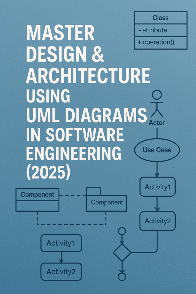
Design Architecture using UML Diagrams in Software Engineering : When it comes to building robust and maintainable software, having a clear understanding of design and architecture is crucial. The design phase translates system requirements into a blueprint, laying the foundation for code development. Architecture, on the other hand, outlines the overall structure and behavior of the system, ensuring it can meet both functional and non-functional requirements efficiently.
One powerful tool used in software design and architecture is the Unified Modeling Language (UML). UML provides a standard way to visualize the design of a system through different types of diagrams, each representing different aspects of the system. In this article, we will dive into four essential UML diagrams—Use Case, Class, Sequence, and Activity Diagrams—to understand how they help in the design and architecture of software systems.
Master Design Architecture using UML Diagrams in Software Engineering (2025)
Design Architecture using UML
1. Use Case Diagram
A Use Case Diagram is a visual representation of the system’s functional requirements. It shows the interactions between users (or other systems) and the system itself. These interactions are represented as use cases, which depict specific tasks or operations that the system can perform.
Components:
Actors: Represent the external entities (users or systems) that interact with the system.
Use Cases: Represent the various functions or processes that the system performs in response to the actors’ actions.
System Boundary: Defines the scope of the system, indicating what is inside the system and what lies outside.
Example:
Consider a Library Management System:
Actors: Librarian, Member, Administrator.
Use Cases: Borrow Book, Return Book, Add New Book, Search Catalog, Update Member Information.
The Use Case Diagram for this system would illustrate how each actor interacts with the system and the functionalities they can access.
2. Class Diagram 📦
A Class Diagram is one of the most important diagrams in object-oriented design. It provides a static view of the system by showing the classes, their attributes, methods, and the relationships between them.
Components:
Classes: Represent the objects or entities in the system, defined by their attributes and methods.
Associations: Indicate relationships between classes, such as one-to-one, one-to-many, or many-to-many.
Inheritance: Denotes the relationship where one class (the subclass) inherits attributes and behaviors from another (the superclass).
Multiplicity: Indicates how many instances of a class can be associated with an instance of another class.
Example:
For the Library Management System, the class diagram might include:
Classes: Book, Member, Librarian, Transaction.
Attributes: Book (title, author, ISBN), Member (name, membership ID), Transaction (date, book).
Methods: Borrow(), Return(), Search().
3. Sequence Diagram ⏳
A Sequence Diagram provides a dynamic view of the system by showing how objects interact with each other in a particular scenario over time. It emphasizes the sequence of messages exchanged between objects to achieve a specific functionality.
Components:
Objects: Represent the entities involved in the interaction.
Messages: Represent the interactions between objects, typically method calls or data exchanges.
Lifelines: Vertical dashed lines representing the time span during which an object exists in the interaction.
Activation Bars: Rectangles on the lifeline, showing when an object is active and processing a message.
Example:
In the Library Management System, a sequence diagram might illustrate how a Member interacts with the system to borrow a book:
The Member sends a borrow request to the Librarian object.
The Librarian checks if the book is available.
The Member receives confirmation, and the book is borrowed.
The sequence diagram ensures that the communication flow is understood and accurately modeled for that specific scenario.
4. Activity Diagram 🔄
An Activity Diagram models the workflow or the business process in the system. It shows the flow of control from one activity to another and helps in understanding the sequence of operations or the steps involved in a process.
Components:
Activities: Represent tasks or actions performed in the system.
Transitions: Indicate the flow between activities.
Decision Nodes: Represent points where the flow splits based on a condition.
Start/End Points: Indicate the entry and exit points of the activity.
Example:
For the Library Management System, an activity diagram for borrowing a book might include:
Start: The member logs into the system.
Decision: Check if the book is available.
Yes: Proceed to borrow.
No: End.
Borrow Book: The system processes the borrow request.
End: The transaction is complete.
Why Use UML Diagrams in Software Design?
Visualization: UML diagrams provide a clear, graphical representation of a system, making it easier for stakeholders to understand the system’s design and architecture.
Communication: They serve as a common language between developers, business analysts, designers, and clients, ensuring everyone is aligned.
Documentation: UML diagrams help in documenting the design process, providing valuable references for future development or maintenance.
Problem-solving: These diagrams help identify potential issues early in the design phase by visualizing complex relationships and interactions.
💛 Support Embedded Prep
If you find our tutorials helpful and want to support our mission of sharing high-quality embedded system knowledge, you can contribute by buying us a coffee.
Every small contribution helps us keep creating valuable content for learners like you. ☕
Thank you for your support — it truly keeps Embedded Prep growing. 💻✨
UML State Machine Diagrams
In software and systems design, understanding how an object behaves in response to different events is crucial. This is where UML State Machine Diagrams come into play. These diagrams visualize how an object changes state based on events, helping designers model dynamic behaviors effectively.
What is a UML State Machine Diagram?
A UML (Unified Modeling Language) State Machine Diagram—also known as a statechart diagram—is used to describe the lifecycle of an object. It shows:
Different states an object can occupy.
Transitions between states triggered by events.
Actions executed during state changes or while in a state.
These diagrams are particularly useful in real-time systems, embedded systems, protocols, workflow modeling, and any domain where the object’s state plays a key role.
Key Concepts and Terminology
1. State
A condition or situation during the life of an object where it satisfies some condition or waits for an event.
Initial State: Represented by a filled black circle (●). It marks the starting point of the state machine.
Final State: Represented by a bullseye (◎). It indicates the end of the object’s lifecycle.
Composite State: A state that contains sub-states, useful for representing complex behavior.
Substate: A state nested inside a composite state.
2. Transition
A directed arrow (→) that shows the movement from one state to another. It typically includes:
Event [Guard] / Action
Event: The trigger for the transition.
Guard (optional): A condition that must be true for the transition to occur.
Action (optional): An operation that occurs during the transition.
3. Action vs Activity
Action: Executes instantaneously as a result of a transition.
Activity: Represents longer-running behavior during a state.
Once Pushed in the Unlocked state, it goes back to Locked.
When to Use State Machine Diagrams
Use state machine diagrams when:
Modeling reactive systems that respond to external/internal events.
Describing workflow systems, like approval processes or UI interactions.
Visualizing protocols or communication sequences.
Implementing finite state machines (FSMs) in embedded systems.
Best Practices
Keep states simple and meaningful.
Use guard conditions to handle conditional transitions.
Prefer entry/exit actions for reusable logic.
Break down complex systems using composite states.
Ensure completeness—every event in a state should be handled or explicitly ignored.
Tools That Support UML State Diagrams
Popular modeling tools include:
Visual Paradigm
Lucidchart
StarUML
Enterprise Architect
Draw.io
These tools often support code generation for certain languages based on the state machine logic.
Understanding Finite State Machines (FSM)
In computing and electronics, Finite State Machines (FSMs) are fundamental models used to design systems that react to inputs based on their current state. From vending machines to traffic lights and embedded systems, FSMs power countless real-world applications.
What is a Finite State Machine?
A Finite State Machine (FSM) is a computational model consisting of a finite number of states, transitions between those states, inputs that trigger transitions, and optional outputs. At any given time, the system is in exactly one state, and changes to another state based on inputs and predefined rules.
Key Components of FSM
States: The various modes in which the machine can exist (e.g., Idle, Running, Stopped).
Initial State: The state where the system starts.
Input: External data or events that trigger state transitions.
Transition Function: Rules that define how the system moves from one state to another based on input.
Final (Accepting) State(optional): A special state that indicates completion or acceptance.
Output(for Mealy/Moore machines): The actions produced by the machine depending on its state or transition.
Types of Finite State Machines
1. Moore Machine
Output depends only on the current state.
Output is associated with the state.
2. Mealy Machine
Output depends on both the current state and the input.
Output is associated with transitions.
Feature
Moore Machine
Mealy Machine
Output
Based on state
Based on state + input
Simplicity
Easier to design and debug
More responsive
States
May require more states
Can be more compact
Real-World Example: Traffic Light Controller
States:
Green
Yellow
Red
Input:
Timer
FSM Logic:
Start in Red.
After timer expires, go to Green.
Then Yellow.
Then back to Red.
Transition Table:
Current State
Input (Timer)
Next State
Output
Red
Expired
Green
Go
Green
Expired
Yellow
Slow Down
Yellow
Expired
Red
Stop
Applications of FSM
FSMs are used in a wide variety of domains:
Embedded Systems: Control units, protocol design, device firmware.
Game Development: NPC behaviors, game states (e.g., Start, Play, Pause, Game Over).
UI Navigation: Button clicks, menu transitions.
Digital Circuits: Sequential logic design using flip-flops.
Compilers: Lexical analysis using deterministic FSMs (DFAs).
FSM vs UML State Machine Diagram
While both model state behavior, they serve slightly different purposes:
Aspect
FSM
UML State Machine Diagram
Usage
Code-level modeling
High-level design & documentation
Detail Level
Simple state-input-output logic
Detailed with entry/exit actions
Visual Representation
Typically tabular or minimalistic
Rich, diagrammatic (UML-based)
Support for Hierarchy
No (basic FSM)
Yes (composite, nested states)
Benefits of Using FSMs
Predictable Behavior: Every input has a well-defined outcome.
Modularity: Easy to extend and maintain.
Formal Verification: Well-suited for testing and validation.
Code Generation: FSMs can be translated into actual program logic easily.
FSM in Embedded C Example
typedef enum { RED, GREEN, YELLOW } State;
State currentState = RED;

void timerExpired() {
    switch (currentState) {
        case RED: currentState = GREEN; break;
        case GREEN: currentState = YELLOW; break;
        case YELLOW: currentState = RED; break;
    }
}
Software Architecture Patterns
When building software — whether it’s a web app, an embedded system, or a desktop application — organizing the code in a clean, scalable way is critical. That’s where Software Architecture Patterns come into play.
Let’s explore the most common patterns:
1. Layered Architecture (aka n-tier Architecture)
What It Is:
This pattern organizes the system into layers. Each layer has a specific responsibility and only communicates with adjacent layers.
Typical Layers:
Presentation Layer – UI, user interaction
Application Layer – Coordinates business logic
Business Logic Layer – Implements core rules and logic
Data Access Layer – Handles storage and retrieval
Example:
Imagine a simple banking app:
The UI shows account balance (Presentation)
It asks the application layer to fetch it
Business logic layer checks if the user is authenticated
Data access layer gets balance from the database
Pros:
Easy to understand and maintain
Good separation of concerns
Common in enterprise applications
Cons:
Can become rigid; layers depend on each other too much
Might have performance overhead
2. Modular Architecture
What It Is:
Breaks the system into independent modules that can be developed and deployed separately.
Each module has a clearly defined interface and can be reused or swapped without affecting the rest of the system.
Think of it like:
LEGO blocks — you can combine different pieces to build various things.
Example:
In an e-commerce platform:
A Payment Module
A User Authentication Module
A Product Catalog Module
Each can be worked on independently by different teams.
Pros:
High flexibility and reusability
Easier testing and maintenance
Ideal for microservices and plugin-based systems
Cons:
Can be harder to integrate
Requires careful interface design
3. Event-Driven Architecture
What It Is:
The system reacts to events. Components send and listen for events asynchronously.
Example:
In an IoT system:
A sensor detects temperature rise and emits an event
A controller receives the event and turns on a fan
You build a core system and allow new features to be added as plugins without changing the core.
Example:
Think of a media player:
The core handles playback
Plugins add support for MP3, MP4, subtitles, streaming, etc.
Pros:
Very extensible
Good for systems that evolve over time
Cons:
Plugin interactions can get messy
Version management is tricky
5. Microservices Architecture
What It Is:
The application is split into small services, each running independently and communicating via APIs (usually HTTP/REST).
Example:
A ride-sharing app:
A service for user profiles
A service for ride matching
A service for payment processing
Each can be scaled or updated without touching the others.
Pros:
Flexible and scalable
Independent deployment
Cons:
Complex deployment and networking
Requires DevOps maturity
6. Client-Server Architecture
What It Is:
Divides the system into clients (requesters) and servers (responders). The client asks for services; the server provides them.
Example:
A web browser (client) requests a web page from a web server.
Pros:
Simple and widely used
Centralized server simplifies management
Cons:
Server is a single point of failure
Limited scalability unless load-balanced
7. Service-Oriented Architecture (SOA)
What It Is:
An evolution of modular and client-server patterns where services expose well-defined interfaces and are loosely coupled.
It’s the architectural grandparent of microservices.
Example:
A travel booking platform with services for:
Flight booking
Hotel reservation
Customer reviews
Each service communicates via a standard protocol (like SOAP or REST).
Pros:
Reusability of services
Technology-agnostic
Cons:
Can become heavy with enterprise-level tools
More suitable for large applications
Summary Table
Pattern
Best For
Key Benefit
Layered
Web and enterprise apps
Clear separation of concerns
Modular
Embedded, large systems
High maintainability
Event-Driven
IoT, real-time apps
Decoupling and scalability
Microkernel
Extensible desktop apps
Easy feature addition
Microservices
Scalable cloud apps
Independent deployment
Client-Server
Web systems, databases
Centralized control
Service-Oriented (SOA)
Enterprise systems
Reusable, loosely coupled services
When to Use Which?
Use Layered if you’re starting small and want structure.
Use Modular when building for flexibility and reuse.
Use Microservices if scaling and team independence matter.
Use Event-Driven for responsive, real-time behavior.
Use Microkernel when plugins/extensions are core to your product.
Use Client-Server for simple request-response setups.
Use SOA for interoperable services in enterprise ecosystems.
Where We Design Architecture for Embedded and Real-Time System Design Concepts
Designing the architecture for embedded and real-time systems is a foundational step that determines how reliable, efficient, and responsive your system will be. Whether you’re building a microwave controller or an automotive ECU (Electronic Control Unit), understanding where and how the architecture is designed is crucial.
Let’s explore this step by step in a clear and beginner-friendly way.
What Is System Architecture?
System architecture is a high-level blueprint of how your system will work. It defines:
What components your system will have (e.g., sensors, processors, actuators)
How these components interact
What software modules are needed
How timing, memory, and communication will be handled
Think of it as drawing the floor plan before constructing a building. It helps avoid chaos later.
Where Does Architecture Design Fit in the Development Process?
Architecture design is done early in the development lifecycle, right after requirements are gathered. Here’s a simplified flow:
Communication methods (Bluetooth, Ethernet, Wi-Fi)
Why important?
This hardware becomes the foundation your software will run on
Incorrect hardware decisions can lead to major rework
2. Software Architecture Design
Where?
On UML tools (like Enterprise Architect, Lucidchart, or Visual Paradigm)
In spreadsheets, flowcharts, or even code comments (early drafts)
Often documented in Software Architecture Documents (SAD)
What is decided?
Operating system: Bare-metal or RTOS (like FreeRTOS, QNX, VxWorks)
Task or thread design: What tasks run, their priority, timing, and how they communicate
Driver layers: HAL (Hardware Abstraction Layer), Middleware
Application logic: State machines, interrupt handling, timers
Memory map and stack/heap size
Error handling, watchdog, fault tolerance
Why important?
Ensures that real-time constraints (deadlines) are met
Prevents bugs due to race conditions, priority inversion, or memory issues
Example: Real-Time Temperature Monitoring System
Let’s imagine designing the architecture for a system that reads temperature every second and triggers a fan if it crosses a threshold.
Hardware Architecture:
Microcontroller: STM32F103 (ARM Cortex-M3)
Sensor: DHT11
Fan: Controlled by relay
Power: 5V battery
Software Architecture:
RTOS: FreeRTOS
Tasks:
ReadTempTask: Reads temperature every 1 sec
ControlFanTask: Checks temp and turns fan ON/OFF
Communication: Queues between tasks
Watchdog Timer: Ensures system restarts if a task hangs
Key Concepts in Real-Time Architecture Design
Concept
Meaning
Why It Matters
Task Scheduling
How tasks are run and switched
Ensures real-time deadlines
Inter-task Communication
How tasks talk (queues, semaphores)
Avoids data corruption
Interrupt Handling
Responding to external events
Needs to be fast and safe
Memory Management
RAM, stack, heap usage
Prevent crashes and overflows
Determinism
Predictable execution timing
Core to real-time guarantees
Common Mistakes in Architecture Design
Not considering real-time constraints early
Overloading the main loop without RTOS
Using too much memory or dynamic allocation
No fallback or error handling
Poor separation between hardware and application logic
Tools That Help Design Architecture
Purpose
Tool Examples
Drawing Diagrams
Lucidchart, Draw.io, Microsoft Visio
UML & Modeling
Enterprise Architect, Modelio
Hardware Design
KiCAD, Altium, Proteus
Real-time Modeling
Simulink, Rhapsody
Code & Documentation
Doxygen, Git, VS Code
Conclusion
Designing the architecture for embedded and real-time systems is not just a planning step—it’s the foundation for everything that follows. Whether you’re working with a simple microcontroller or a complex automotive system, good architecture:
Saves time
Reduces bugs
Ensures deadlines are met
Makes your system scalable and maintainable
Start simple, think in blocks, document your design, and always validate your real-time needs.
You can also Visit other tutorials of Embedded Prep
Git Basics : In this blog post, we will dive deep into the core concepts of Git, one of the most widely used version control systems in modern software development. Whether you’re a beginner or looking to brush up on Git, this guide will help you understand how to efficiently manage and track your codebase.
We’ll start by covering the Git Basics such as cloning repositories, committing changes, pushing and pulling updates, and how these foundational commands are used in everyday development. After that, we’ll explore the power of Branching and Merging, which enables parallel development on separate features or fixes without disrupting the main codebase.
Next, we will dive into Git Workflow and examine popular strategies like Feature Branch Workflow and Git Flow, and explore the commands necessary to follow these workflows effectively. We’ll also tackle Conflict Resolution — a common challenge when collaborating with others — and provide best practices for resolving merge conflicts.
Furthermore, we will compare Git Rebase vs Merge, and understand their differences, use cases, and impact on project history. Finally, we will wrap up with Git Tags and Releases, showing how to mark specific points in your project’s history, such as version releases, and how to manage them with tags.
By the end of this post, you’ll have a solid understanding of Git’s key features and commands, enabling you to collaborate smoothly in any software development project.
1. Git Basics Overview:
Git is a distributed version control system that helps developers manage and track changes to their codebase over time. It allows multiple users to collaborate on the same project without overwriting each other’s changes. Below are the basic Git commands that are commonly used in any development project.
Clone: git clone is used to create a local copy of a remote repository. This command pulls down all the files, commit history, and branches from the remote repository to your local machine. git clone <repository_url> Example: git clone https://github.com/user/project.git
Commit: A commit represents a snapshot of your changes. After modifying files in your working directory, you need to add them to staging and commit them to the local repository.
Stage files: git add <file> adds specific files to the staging area. To add all changed files, use git add .. git add .
Commit changes: Once your files are staged, you use the git commit command to save your changes to the local repository. git commit -m "Commit message describing changes"
Push: The git push command is used to upload local repository content to a remote repository. It is typically used after committing changes locally to push them to a shared remote repository. git push origin <branch_name> Example: git push origin main
Pull: git pull is used to fetch and integrate changes from the remote repository into your local branch. This command combines git fetch and git merge, ensuring you have the latest changes from the remote branch. git pull origin <branch_name> Example: git pull origin main
Branching & Merging
2. Branching:
Branching allows you to create separate environments to work on different features or fixes without affecting the main codebase. Each branch can be developed independently and then merged back into the main branch.
Create a branch: You can create a new branch with the git branch command. git branch <branch_name> Example: git branch feature/new-feature
Switch to a branch: To start working on a branch, use git checkout to switch to it. git checkout <branch_name> Example: git checkout feature/new-feature Alternatively, you can combine both creating and switching with: git checkout -b <branch_name> Example: git checkout -b feature/new-feature
3. Merging:
Merging is the process of bringing together changes from different branches. Typically, changes from a feature branch are merged back into the main branch.
Merge a branch: First, ensure you’re on the branch that you want to merge into (typically main or master), then use the git merge command. git merge <branch_name> Example: git merge feature/new-feature
Git Workflow (Feature Branch, Git Flow) and All Commands
4. Git Workflow:
Git workflow refers to how developers manage their branches and commits within a repository. Two popular workflows are the Feature Branch workflow and Git Flow workflow.
Feature Branch Workflow: In this workflow, each new feature or bug fix is developed in a separate branch. When the feature is complete, it’s merged into the main branch. Steps:
Create a feature branch: git checkout -b feature/awesome-feature
Open a pull request (PR) and merge into the main branch.
Git Flow: Git Flow is a more structured branching model, often used in larger projects. It divides work into different branches for features, releases, and hotfixes.
Main branches:
main (or master): Production-ready code.
develop: Ongoing development code, where new features are integrated.
Supporting branches:
Feature branches: Used for new features.
Release branches: Prepare for production releases.
Hotfix branches: Used to fix urgent issues in production.
Git Flow commands: Install git-flow: brew install git-flow Initialize git flow in a repository: git flow init Start a feature: git flow feature start <feature_name> Finish a feature: git flow feature finish <feature_name> Start a release: git flow release start <release_version> Finish a release: git flow release finish <release_version> Start a hotfix: git flow hotfix start <hotfix_version> Finish a hotfix: git flow hotfix finish <hotfix_version>
💛 Support Embedded Prep
If you find our tutorials helpful and want to support our mission of sharing high-quality embedded system knowledge, you can contribute by buying us a coffee.
Every small contribution helps us keep creating valuable content for learners like you. ☕
Thank you for your support — it truly keeps Embedded Prep growing. 💻✨
Conflict Resolution
5. Conflict Resolution:
When merging branches, you might encounter conflicts if two branches modify the same part of a file. Git cannot automatically decide which change should be kept, so it marks the conflict in the file.
Resolve Conflicts: When a conflict occurs, Git will mark the file with conflict markers. Open the conflicted file, look for the markers (e.g., <<<<<<<, =======, >>>>>>>), and manually resolve the conflict by selecting or merging the appropriate changes.
After resolving conflicts: Once you’ve resolved the conflict, stage the file and commit the merge. git add <conflicted_file> git commit
Git Rebase vs Merge
6. Git Rebase vs Merge:
Merge: When you use git merge, you combine the histories of two branches into a single branch. A merge commit is created to maintain the history of both branches.
Pros: Maintains a full history of commits, which can be useful for tracking changes.
Cons: The history can become messy with multiple merge commits.
git merge <branch_name>
Rebase: git rebase moves or “replays” your commits from one branch onto another. It results in a cleaner history without merge commits.
Pros: Creates a linear history.
Cons: Can rewrite history, which might be problematic for shared branches.
git rebase <branch_name>
Git Tags and Releases
7. Git Tags and Releases:
Git tags are used to mark specific points in history, often used for releases. A tag points to a particular commit, allowing you to easily identify and reference a release.
Create a tag: Tags are typically created at significant points in a project’s development, like when releasing a version. git tag -a <tag_name> -m "Tag message" Example: git tag -a v1.0 -m "First official release"
Push tags: By default, tags are not pushed to remote repositories. You need to explicitly push tags. git push origin <tag_name> Example: git push origin v1.0
List tags: To view all the tags in a repository: git tag
Checkout a tag: To checkout a specific tag (e.g., a previous release): git checkout <tag_name> Example: git checkout v1.0
Releases: Releases in GitHub or GitLab use tags to provide a versioned snapshot of the code. When creating a release, you can associate it with a tag to specify the version being released.
Step 1: Set up a Remote Repository
To start, we’ll assume there’s a Git repository already hosted on a platform like GitHub or GitLab (you can create one there if needed).
For this example, the URL for the remote repository is:
https://github.com/username/SampleProject.git
Step 2: Clone the Repository
First, we’ll clone the remote repository to create a local copy.
After this, a new folder SampleProject will be created, and it will contain the files from the remote repository.
Step 3: Create a New Branch for Feature Development
Now that we have the repository, let’s create a new branch to work on a new feature. We’ll call this branch feature/add-new-feature.
cd SampleProject
git checkout -b feature/add-new-feature
The -b flag creates and checks out the new branch.
Step 4: Modify Files and Commit Changes
Let’s assume we add a new file or modify an existing one. For this example, we’ll modify a file called README.md.
Open README.md and add a line like: This is a new feature added to the project.
After saving the file, we need to stage the changes and commit them.
git add README.md  # Stage the file
git commit -m "Add new feature description to README"
This command stages the changes and commits them with a descriptive message.
Step 5: Push the Branch to Remote Repository
Now that the feature is ready, let’s push the feature/add-new-feature branch to the remote repository.
git push origin feature/add-new-feature
This uploads your local branch to the remote repository, making it available for collaboration or review (such as in a pull request).
Step 6: Create a Pull Request (Optional)
If you’re working with a team, you would now go to the remote Git hosting platform (e.g., GitHub) and create a Pull Request (PR) to merge feature/add-new-feature into the main branch.
Step 7: Pull Latest Changes from the Remote Repository
While working on your feature, others may have pushed changes to the remote repository. To keep your local repository up to date, you can pull the latest changes from the main branch.
git checkout main        # Switch to the main branch
git pull origin main      # Pull latest changes from remote main branch
Step 8: Merge the Feature Branch into Main
Once the feature is approved (e.g., through a PR review), you can merge it back into the main branch. If you have already completed the PR, you’d merge the branches from the Git hosting platform interface. However, let’s do it manually on the command line:
git checkout main                  # Switch to the main branch
git merge feature/add-new-feature   # Merge feature branch into main
At this point, your main branch includes the changes from feature/add-new-feature.
Step 9: Resolve Merge Conflicts (If Any)
If changes in the main branch and feature/add-new-feature branch conflict (e.g., both modified the same line in README.md), Git will mark the file as conflicted, and you’ll need to resolve the conflict.
You’ll see conflict markers in the file, like:
<<<<<<< HEAD
This is the content from the main branch.
=======
This is the content from the feature branch.
>>>>>>> feature/add-new-feature
You manually edit the file to keep the desired changes and remove the markers.
GDB GNU Debugger : GDB is a powerful tool used by developers to inspect what’s going on inside a running program or after it crashes. It helps you find and fix bugs by allowing you to pause execution, examine variables, inspect memory, and even step through lines of code.
The GNU Debugger (GDB) is a powerful tool used to debug programs written in various programming languages. It lets you inspect and modify memory, control the execution flow, set breakpoints, and much more to analyze and fix issues in your code.
GDB GNU Debugger
1. Installing GDB
In Red Hat Developer Toolset, the GNU Debugger is part of the devtoolset-9-gdb package, and it’s automatically installed along with the toolset. To get started with GDB, follow these installation steps:
If you’re using the devtoolset-9 toolchain, GDB is already included. Here’s how you can install the necessary packages:
To start debugging your program with GDB, use the following command:
$ scl enable devtoolset-9 'gdb fibonacci'
Once inside GDB, you’ll see a prompt where you can start debugging your program. To exit GDB, simply type:
(gdb) quit
4. Listing Source Code
To view the source code of the program you’re debugging, use the list command in GDB. It will show the first 10 lines of the code. You can also change the number of lines displayed:
(gdb) list
(gdb) set listsize 20  # Show 20 lines instead of 10
5. Setting Breakpoints
A breakpoint is a place where the program will stop, allowing you to inspect the state of your program. You can set a breakpoint at a specific line or function:
Once you’ve set breakpoints, you can run your program inside GDB:
(gdb) run
If your program needs arguments, you can pass them like this:
(gdb) run arg1 arg2
The program will stop at the first breakpoint or when it encounters an error.
7. Displaying Variable Values
To check the current value of a variable while debugging, use the print command:
(gdb) print variable_name
For example, after stopping at a breakpoint, you can print the value of a variable:
(gdb) print a
(gdb) print b
8. Continuing Execution
To continue the program after hitting a breakpoint, use the continue command:
(gdb) continue
If you want to skip a certain number of breakpoints or stop after a few lines of code, use:
(gdb) continue number
(gdb) step number
The step command allows you to execute a specific number of lines, which is useful when you’re debugging loops or functions.
Example Workflow
Compile the Program with Debug Info:$ scl enable devtoolset-9 'gcc -g -o fibonacci fibonacci.c'
Start Debugging with GDB:$ scl enable devtoolset-9 'gdb fibonacci'
Set Breakpoint at Line 10:(gdb) break 10
Run the Program:(gdb) run
Print Variable Values:(gdb) print a (gdb) print b
Continue Execution:(gdb) continue
Let’s work with a simple C code example to demonstrate the use of GDB.
Example C Program: factorial.c
#include <stdio.h>

int factorial(int n) {
    if (n == 0 || n == 1) {
        return 1;
    }
    return n * factorial(n - 1);
}

int main() {
    int num = 5;
    int result = factorial(num);
    printf("Factorial of %d is %d\n", num, result);
    return 0;
}
This program calculates the factorial of 5 and prints the result.
Steps to Debug Using GDB:
Compile the Program with Debug Information
To compile the C code with debugging symbols, we use the -g option in gcc.
gcc -g -o factorial factorial.c
This will produce an executable file named factorial.
Start GDB
To start GDB with the compiled program, use the following command:
gdb ./factorial
Set Breakpoints
We want to set a breakpoint at the factorial function to see the recursive calls.
To set a breakpoint at the factorial function, run the following in the GDB prompt:
(gdb) break factorial
Run the Program
Now, run the program inside GDB:
(gdb) run
The program will start, and GDB will pause at the first call to factorial.
Step Through the Code
To step through the code one line at a time, use the step command:
(gdb) step
This will take you inside the factorial function, and you can continue stepping through the function’s execution.
Display Variable Values
To check the value of the variables, such as n, you can use the print command. For example:
(gdb) print n
This will show the value of n at each step of the recursion.
Continue Execution
After reaching the breakpoint and checking variable values, you can continue execution until the next breakpoint (or the end of the program):
(gdb) continue
Exit GDB
Once you’re done, exit GDB by typing:
(gdb) quit
Expected Output
During the debugging session, GDB will allow you to inspect the recursive calls to factorial and the values of n at each step. Eventually, it will display the final result after the program reaches the print statement.
1. GDB Basics and Commands
What is GDB?
GDB is the GNU Debugger. It lets you:
Start your program and pause it anywhere.
View variable values at runtime.
Step through code line by line.
Set breakpoints (pause points).
Inspect memory and CPU registers.
How to Compile with Debug Info
Before using GDB, compile your code with debug symbols:
gcc -g main.c -o main
The -g flag tells the compiler to include debug information.
Starting GDB
gdb ./main
Common Commands
Command
Description
run
Starts the program
break <line/function>
Sets a breakpoint
next or n
Steps to next line (skips function calls)
step or s
Steps into a function
continue or c
Resumes execution
print <var>
Prints the value of a variable
list
Shows source code
quit
Exits GDB
2. Remote Debugging with GDB
Remote debugging is used to debug a program running on another system (like embedded Linux or RTOS).
Setup
On Target (with GDB server):
gdbserver :1234 ./app
On Host (your PC):
gdb ./app
(gdb) target remote <target-ip>:1234
Now you’re controlling the target program from your host machine.
3. Breakpoints, Watchpoints, Backtrace
Breakpoints
Stop execution at specific lines or functions:
(gdb) break main
(gdb) break 42  # line 42
Watchpoints
Automatically pause when a variable changes:
(gdb) watch counter
Backtrace
See the function call history (call stack):
(gdb) backtrace
This shows which functions were called and in what order.
4. Disassembly and Register Inspection
Disassemble Code
See the machine code for your program:
(gdb) disassemble main
View Registers
See CPU register values (great for low-level debugging):
(gdb) info registers
For ARM/MIPS/other architectures, you’ll see general-purpose and special registers.
5. Debugging on Bare-Metal & RTOS
Bare-Metal Debugging
Bare-metal means there’s no OS — you’re debugging directly on hardware (e.g., ARM Cortex-M microcontroller).
RTOS debugging is similar to bare-metal, but you may need:
RTOS-aware GDB scripts (for thread/task context)
Special memory maps
You can:
Pause execution
View current tasks
Inspect stack of each thread
GDB extensions/plugins like FreeRTOS-aware GDB scripts can show tasks and queues.
How GDB Interacts with Compiled Binaries
GDB (GNU Debugger) is a tool used to examine and control programs after they are compiled. When you compile a program, the compiler turns your human-readable source code into machine-readable binary code. GDB interacts with these compiled binaries by reading and controlling their execution.
Here’s how it works step-by-step:
Reading the Binary File GDB loads the compiled binary file (usually an executable) into memory. If the binary contains debugging information (generated using the -g flag during compilation), GDB can use this information to map machine code back to your original source code, including variables, functions, and line numbers.
Connecting to the Process GDB can either start a program directly or attach to an already running process. It uses system-level APIs to take control of the process execution.
Controlling Execution Once attached, GDB can pause program execution (breakpoints), step through code line-by-line (step/next), or continue execution. This allows programmers to inspect exactly how their code is running.
Inspecting Memory and Variables GDB reads the memory and register states of the running program. This lets you examine variable values, memory contents, and CPU registers to understand the program’s behavior.
Modifying Execution GDB can also change variable values, set new program counter positions, or modify registers while the program runs. This helps in testing fixes without recompiling.
Key takeaway: GDB bridges the gap between your compiled binary and the original source code, allowing you to inspect, control, and debug the program’s execution at a very deep level.
Breakpoints and Watchpoints in GDB
When debugging with GDB, you often need to pause the program or observe certain events to understand its behavior. That’s where breakpoints and watchpoints come in. They are both tools to stop or monitor a program during execution, but they work differently.
1. Breakpoints
A breakpoint is a marker you set at a specific line of code or function. When the program execution reaches that point, GDB pauses the program so you can inspect the state of the program.
Example use case: If your program crashes in a function, you can set a breakpoint at the function start to see exactly what happens before the crash.
How to set a breakpoint in GDB:
(gdb) break main   # Break at the start of main()
(gdb) break 25     # Break at line 25 in the current file
When the program hits the breakpoint, GDB stops execution and gives control back to you.
2. Watchpoints
A watchpoint is like a dynamic watch on a variable or memory location. GDB pauses execution whenever the value of that variable or memory changes.
Example use case: If a variable is changing unexpectedly, you can set a watchpoint on it to find the exact point where the change happens.
How to set a watchpoint in GDB:
(gdb) watch x # Watch variable x
When the watched variable changes, GDB stops execution and shows where the change occurred.
Key Differences Between Breakpoints and Watchpoints
Feature
Breakpoint
Watchpoint
Purpose
Stop execution at a specific line or function
Stop execution when a variable or memory changes
Trigger
Reaching a specific location in code
Change in the value of a variable or memory
Usage
Used to inspect execution flow
Used to monitor specific variable changes
Performance
Low impact on performance
Higher performance cost because memory is monitored
In short:
Breakpoints → Stop at a specific point in code.
Watchpoints → Stop when data changes.
Summary
Feature
GDB Command
Set Breakpoint
break <line/function>
Step Through Code
next, step
Inspect Variable
print var
Remote Debug
target remote <ip:port>
View Registers
info registers
Disassemble
disassemble
Watch Variable
watch var
Backtrace
backtrace
Here’s a beginner-friendly, plagiarism-free, and uniquely written explanation of essential GDB commands, complete with simple descriptions and a few helpful tips.
Common GDB Commands You Should Know
Command
What It Does (Beginner-Friendly)
run or r
Starts the program from the beginning. Great for testing your code cleanly.
break or b
Puts a stop (breakpoint) at a specific line or function so you can pause there.
disable
Temporarily turns off a breakpoint without removing it. Useful for quick toggles.
enable
Turns a disabled breakpoint back on. Handy if you’re toggling breakpoints often.
next or n
Moves to the next line of code without entering into any called function.
step
Goes to the next line, but enters into functions to help debug them deeper.
list or l
Shows the source code around the current line or a specified location.
print or p
Shows the current value of a variable. Also great for checking expressions.
quit or q
Exits GDB. You’ll be asked to confirm if the program is still running.
clear
Removes all breakpoints, or just one if specified. Good for cleanup.
continue
Resumes program execution after hitting a breakpoint or stepping through code.
Example Session (Simple Workflow)
$ gdb ./my_program     # Start GDB with your compiled program
(gdb) break main       # Set a breakpoint at the beginning
(gdb) run              # Start running the program
(gdb) next             # Move to the next line
(gdb) print myVar      # Check the value of a variable
(gdb) continue         # Resume execution until next breakpoint
(gdb) quit             # Exit when you're done
Frequently Asked Questions (FAQ)
1. What is GDB and why is it used?
GDB (GNU Debugger) is a powerful debugging tool used to analyze and debug programs written in languages like C, C++, and others. It helps developers inspect code, find bugs, check variable values, trace program execution, and understand crashes or unexpected behavior.
2. Is GDB only for C/C++ programs?
No! While GDB is widely used for C and C++, it also supports other languages like Ada, Fortran, Go, Rust, and more—depending on compiler support and integration.
3. How do I install GDB?
Linux: Use your package manager (e.g., sudo apt install gdb on Ubuntu).
macOS: Use Homebrew → brew install gdb.
Windows: Install via MinGW or download pre-built binaries from official sites.
4. Can GDB debug running processes?
Yes! GDB can attach to an already running process using the attach <pid> command, allowing you to debug without restarting the application.
5. What are breakpoints in GDB?
Breakpoints are markers you set in code to pause execution at specific lines or functions. They let you inspect program state, variables, and execution flow at precise points.
Example:
(gdb) break main
6. How do I run a program inside GDB?
Use the run command:
(gdb) run
Or pass arguments like:
(gdb) run arg1 arg2
7. What is a backtrace in GDB?
A backtrace (via the bt command) shows the call stack leading to the current point in execution. It’s very helpful for diagnosing where and how a program crashed.
8. Can GDB be used for remote debugging?
Yes. GDB supports remote debugging over serial ports, TCP/IP, or JTAG interfaces. You use target remote to connect to a remote GDB server.
9. Is GDB suitable for beginners?
Absolutely! While it has a learning curve, GDB is beginner-friendly once you grasp basic commands like break, run, next, step, print, and bt.
10. Are there graphical front-ends for GDB?
Yes. Tools like:
DDD (Data Display Debugger)
Eclipse CDT Debugger
Insight
GDB Dashboard (TUI enhancements)
These provide graphical interfaces that make debugging visually easier.
11. How can I debug core dumps with GDB?
If your program crashes and generates a core file, you can inspect it like this:
gdb <program> core
This lets you analyze the state of the program at the time of the crash.
12. Is GDB available for free?
Yes! GDB is completely free and open-source, distributed under the GNU General Public License (GPL).
13. What’s new in GDB for 2025?
(Replace this with your blog’s content if you’ve covered new GDB updates. For example:)
JTAG stands for Joint Test Action Group, which is the name of the group that initially developed the standard. Today, JTAG commonly refers to both the group and the test interface and protocol defined by the IEEE 1149.1 standard.
Originally created in the 1980s, JTAG was developed as a solution to a growing problem in electronics manufacturing: how to test complex circuit boards where physical access to all the pins and components was no longer possible.
Why Was JTAG Created?
As electronic components became smaller and more integrated, traditional testing methods like bed-of-nails testers or external probes couldn’t easily reach the pins or internal signals of components. JTAG was introduced to allow:
Testing of individual pins and board connections,
Debugging of embedded systems,
Programming of microcontrollers, FPGAs, CPLDs, and flash memory,
Diagnosing faults during development and manufacturing.
JTAG Is More Than Just Debugging and Programming
When most people think of JTAG, they associate it with debugging processors or programming FPGAs and CPLDs. That’s not wrong—but it’s only part of the story.
JTAG isn’t just about debugging. It isn’t just about programming either.
While you might know JTAG through tools that connect to a JTAG interface, such as debuggers or flash programmers, those tools typically use only one part of what JTAG has to offer: the four-wire communication protocol defined by the IEEE 1149.1 standard.
What Else Can JTAG Do?
JTAG was originally developed as a solution for testing circuit boards—specifically to overcome the limitations of traditional test methods like bed-of-nails testers. These older methods required physical access to every pin or needed complex custom setups for functional testing.
To solve this, IEEE created the concept of a Test Access Port (TAP), which uses four signals (TCK, TMS, TDI, TDO) to interact with special test registers inside chips.
The key test register introduced by this standard is the Boundary Scan Register (BSR).
What Is a Boundary Scan Register?
The Boundary Scan Register sits at the edges (or “boundaries”) of a chip, between its functional logic core and the actual pins that connect it to a board. That’s why JTAG testing is often called “boundary scan” testing.
These registers are made up of individual cells that can:
Operate in functional mode, where they don’t interfere with normal chip behavior.
Operate in test mode, where they take control of the chip’s input/output pins.
In test mode, these boundary scan cells allow us to:
Drive specific values onto the board’s signal lines (outputs),
Read the values present on those lines (inputs).
How Does This Help in Testing?
Here’s the powerful part: When JTAG is used in test mode, it allows engineers to control and observe signals on a PCB without booting the system or loading firmware. The device doesn’t need to be configured—it just needs to support boundary scan.
This means:
You can test for short circuits, opens, and miswirings,
You can run tests without needing full firmware or software,
It reduces the need for physical access to test points.
Two Main Ways to Use JTAG for Testing
Connection Testing This basic method checks for short circuits and open connections by using only the JTAG-capable devices and their pins. It provides good coverage using the board’s layout and JTAG features.
Extended Testing (with non-JTAG devices) Tools like XJTAG can go further by using JTAG-enabled chips to talk to non-JTAG devices (e.g., DDR RAM, Flash). This allows testing of more complex components using the existing JTAG infrastructure.
JTAG is much more than a tool for programming chips or debugging firmware. It’s a powerful hardware test interface that helps engineers:
Test boards without physical probes,
Check soldering and connectivity,
Debug hardware issues early in development,
Communicate with various components through a simple 4-pin interface.
So next time you hear “JTAG,” remember: It’s not just a port—it’s a gateway to deep-level access and testing.
💛 Support Embedded Prep
If you find our tutorials helpful and want to support our mission of sharing high-quality embedded system knowledge, you can contribute by buying us a coffee.
Every small contribution helps us keep creating valuable content for learners like you. ☕
Thank you for your support — it truly keeps Embedded Prep growing. 💻✨
1. Introduction
When working with embedded systems, hardware debugging, or board-level testing, JTAG is a name that comes up often. But what exactly is it?
JTAG stands for Joint Test Action Group—the name of the group that developed the standard. It’s an interface and protocol that allows you to test, debug, and program devices on a circuit board, even when they are soldered down and inaccessible through traditional means.
2. What is JTAG?
At its core, JTAG is a standard for verifying designs and testing printed circuit boards (PCBs) after manufacture. It provides a standardized interface to communicate with chips using just a few pins.
JTAG was standardized as IEEE 1149.1 in 1990 and is commonly used in embedded systems, FPGA programming, microcontroller debugging, and boundary scan testing.
3. Why Was JTAG Introduced?
Before JTAG, engineers used bed-of-nails testers or manually probed signals on PCBs. These methods had major drawbacks:
JTAG solved this by embedding test logic inside chips, allowing for internal signal monitoring and control through a serial interface—no need to physically touch internal nodes!
4. How Does JTAG Work?
JTAG enables access to a device’s internal functions using a serial protocol and a Test Access Port (TAP). This port can:
Control internal registers
Access memory
Perform boundary scans
Program flash memory
The TAP connects to a chain of devices called a JTAG daisy chain. Devices in the chain share the same control signals, but each has its own data path.
The core components inside a JTAG-enabled device include:
TAP Controller – Controls the JTAG state machine
Instruction Register (IR) – Decides what operation to perform (e.g., read ID, boundary scan)
Data Registers (DR) – Used to shift in/out data
5. JTAG Pinout and Signals
JTAG usually uses 4 or 5 pins:
Pin Name
Full Form
Description
TDI
Test Data In
Serial data input into the JTAG chain
TDO
Test Data Out
Serial data output from the JTAG chain
TCK
Test Clock
Provides the clock for synchronizing data
TMS
Test Mode Select
Controls the state of the TAP controller
TRST
Test Reset (optional)
Resets the JTAG state machine (not always used)
6. Common Use Cases of JTAG
Boundary Scan Testing
Check connectivity between pins and trace faults without physical probing.
In-System Programming (ISP)
Program flash memory, FPGAs, CPLDs, and MCUs via JTAG.
Debugging Embedded Systems
Set breakpoints, inspect registers, view memory, and single-step through code.
Hardware Bring-Up
Access low-level hardware registers before firmware is ready.
7. JTAG in Embedded Systems
JTAG is essential for developers working on ARM Cortex, STM32, ESP32, or custom SoCs. It allows you to:
Flash firmware without bootloader
Debug without printf()
Perform post-silicon validation
Example: JTAG with STM32
Using an ST-Link or J-Link programmer, you can connect to the STM32 via JTAG or SWD (Serial Wire Debug, a 2-wire variant) and debug using tools like OpenOCD + GDB or STM32CubeIDE.
8. Tools and Software for JTAG
Hardware Debug Probes:
SEGGER J-Link
ST-Link (for STM32)
TI XDS110 (for TI MCUs)
FTDI-based cables (DIY options)
Software:
OpenOCD (Open On-Chip Debugger) – Popular open-source JTAG interface
GDB – GNU debugger for step-through debugging
Vendor IDEs – STM32CubeIDE, IAR, Keil MDK, Code Composer Studio
9. Advantages and Limitations
Advantages
Access internal registers and memory
Non-intrusive testing and debugging
Programming without bootloader
Works even when the system is not fully booted
Limitations
Not supported by all chips
Configuration can be complex for beginners
Risk of bricking if improperly used
JTAG interfaces can be disabled for security in some products
10. Conclusion
JTAG is a powerful and essential interface for hardware debugging, device testing, and embedded system development. While it may seem complex at first, learning JTAG opens the door to low-level system access, deep debugging, and smoother hardware bring-up processes.
If you’re working with microcontrollers, FPGAs, or custom PCBs, understanding JTAG is a must-have skill.
FAQ – Master JTAG (Joint Test Action Group): A Beginner-Friendly, In-Depth Guide (2025)
1. What is JTAG and why should I learn it?
JTAG (Joint Test Action Group) is a standard (IEEE 1149.1) used for testing, programming, and debugging hardware—mainly microcontrollers, FPGAs, and CPUs. Learning JTAG is essential for embedded developers, hardware engineers, and system testers as it gives direct access to chip internals, enabling tasks like:
Boundary-scan testing (fault detection on PCBs)
Flashing firmware directly
Debugging software running on target boards
2. What are the typical use cases of JTAG?
Hardware testing: Identify faulty components or soldering defects.
Firmware flashing: Load firmware into non-volatile memory without a bootloader.
Real-time debugging: Step through code, inspect registers, memory, and control execution.
Board bring-up: Debug and validate hardware during prototype development.
3. Which hardware tools do I need for JTAG?
You typically need:
A JTAG debugger/programmer (e.g., SEGGER J-Link, ST-LINK, OpenOCD-compatible dongles)
A target device that supports JTAG (e.g., STM32, ARM Cortex-M, Xilinx FPGAs)
4. What are the standard JTAG pinouts and signals?
Typical JTAG signals include:
TDI (Test Data In) – Data input to the target
TDO (Test Data Out) – Data output from the target
TCK (Test Clock) – Clock signal
TMS (Test Mode Select) – Controls state transitions
TRST (optional) – Test Reset
GND – Ground
Vref – Reference voltage (for logic level compatibility)
5. How does JTAG work internally?
JTAG uses a TAP controller (Test Access Port), which moves through states based on the TMS and TCK lines. It shifts data into registers (e.g., instruction register, data register) and enables control over internal signals without requiring CPU code execution.
6. Is JTAG only for testing hardware?
No. While JTAG was initially designed for boundary-scan testing, it evolved to support:
Flash programming
Low-level debugging
Chip-level introspection
Reset and boot control
7. Can I use JTAG with open-source tools?
Yes. Tools like:
OpenOCD (Open On-Chip Debugger) for programming and debugging
GDB for source-level debugging with breakpoints and watchpoints
UrJTAG for boundary-scan and low-level testing
These tools are often free and widely supported.
8. What’s the difference between JTAG and SWD (Serial Wire Debug)?
JTAG: 4–5 signals; full IEEE 1149.1 standard; widely supported.
SWD: ARM-specific 2-wire protocol; lighter and faster; used on Cortex-M devices. Both support debugging and programming, but SWD is preferred for space-constrained designs.
9. What are boundary-scan and chain configurations in JTAG?
Boundary-scan: Allows testing of I/O pins without booting the processor.
JTAG chain: Multiple devices can be connected in series (TDI → TDO) using a single JTAG interface. Each device has a unique ID and is accessed through a specific instruction.
10. What are common JTAG errors and how do I fix them?
Error
Cause
Fix
Target not found
Wrong pinout, bad solder
Check wiring, use multimeter
Device ID mismatch
Wrong chip selected
Check chain or update config
No response to TCK/TMS
Dead chip or damaged port
Try alternate device or port
OpenOCD config failed
Wrong interface/chip
Double-check .cfg files
11. Can JTAG be used on production devices?
Yes, but JTAG is often disabled or locked for security reasons in production devices. Secure provisioning may require unlocking or access keys.
12. Where can I practice JTAG debugging hands-on?
Start with:
STM32 Nucleo or Discovery boards
ESP32 DevKit
Raspberry Pi with GPIO for JTAG
FPGAs like Xilinx or Intel (with USB Blaster, Platform Cable)
Use OpenOCD + GDB or manufacturer IDEs (STM32CubeIDE, Xilinx Vivado, etc.).
13. What are the career benefits of learning JTAG?
Mastering JTAG gives you an edge in:
Embedded software development
Board-level diagnostics
Hardware testing and verification
Secure firmware deployment It’s a key skill for Embedded Engineers, Firmware Developers, and Test Engineers.
You can also Visit other tutorials of Embedded Prep
SWD Serial Wire Debug : When working with microcontrollers, debugging is a key part of development. One common way to debug embedded systems is using SWD, short for Serial Wire Debug. It’s a modern, efficient way to communicate with a microcontroller during development.
Let’s break it down in a simple way.
What is SWD Serial Wire Debug?
Serial Wire Debug (SWD) is a two-wire protocol developed by ARM for debugging ARM Cortex-M microcontrollers. It is an alternative to the older JTAG protocol, which uses more pins.
SWD allows you to:
Load firmware into the microcontroller.
Set breakpoints and step through code.
Read and write memory.
Monitor and control the processor state.
SWD Serial Wire Debug vs JTAG
Feature
SWD (Serial Wire Debug)
JTAG
Wires
2
4-5
Speed
Fast
Fast
Pin Usage
Low (good for small MCUs)
Higher (more GPIO needed)
Complexity
Simpler
More complex
Debug Access
Full access
Full access
So, SWD is preferred when you have limited pins available and are working with ARM-based chips.
How SWD Serial Wire Debug Works
SWD uses only 2 main signals:
SWDIO – Serial Wire Debug Input/Output Acts like data line (similar to SDA in I2C).
SWCLK – Serial Wire Clock Acts like the clock line (similar to SCL in I2C).
Optionally, you might also have:
nRESET – To reset the microcontroller from the debugger (optional).
GND – A common ground between your debug tool and target board (mandatory).
Tools Involved
To use SWD, you need:
A microcontroller that supports SWD (e.g., STM32, NXP, etc.).
A debug probe, such as:
ST-Link (for STM32)
J-Link (Segger)
CMSIS-DAP
A debugger software like:
STM32CubeIDE
Keil uVision
OpenOCD with GDB
SWD Serial Wire Debug Pinout Example (STM32)
Here’s a common SWD pinout on STM32 boards:
Pin Name
Function
SWDIO
Data
SWCLK
Clock
GND
Ground
3.3V
Power supply
NRST
Reset (optional)
Why Use SWD?
👨💻 Easy Debugging: Load, step, break, and inspect code easily.
🧠 Access RAM/Flash: Read/write memory and registers.
🔄 Flash Programming: Upload firmware via the debug interface.
📉 Fewer Pins: Perfect for space-constrained designs.
🧰 Low-Cost Tools: Many low-cost debug probes available.
Real-Life Use Case
Let’s say you’re working with an STM32 microcontroller. You want to flash your code and debug it:
Connect ST-Link to SWDIO, SWCLK, GND, and optionally NRST.
Open STM32CubeIDE and start a debug session.
You can now:
Set breakpoints in code.
See variables change in real time.
Step through the program.
Prerequisites
Before you start, make sure you have:
✅ A microcontroller board (e.g., STM32F103, STM32 Nucleo).
✅ A debug probe (e.g., ST-Link, J-Link, or CMSIS-DAP).
✅ A PC with debugging software installed (e.g., STM32CubeIDE, Keil uVision, OpenOCD + GDB).
✅ Wires or a USB cable to connect the debugger.
✅ Basic USB driver for the debug probe installed.
💛 Support Embedded Prep
If you find our tutorials helpful and want to support our mission of sharing high-quality embedded system knowledge, you can contribute by buying us a coffee.
Every small contribution helps us keep creating valuable content for learners like you. ☕
Thank you for your support — it truly keeps Embedded Prep growing. 💻✨
Step-by-Step: Connecting SWD
1. Identify SWD Pins on the Microcontroller
Look for the following pins on your MCU or dev board:
SWDIO – Data line
SWCLK – Clock line
GND – Ground
NRST – (Optional, Reset line)
VCC – Target voltage reference (often 3.3V)
You can find these in the datasheet or board pinout diagram.
2. Connect the Debug Probe
Match these pins between the debugger and the target board:
Debugger Pin
Target Board Pin
SWDIO
SWDIO
SWCLK
SWCLK
GND
GND
NRST (opt.)
NRST
VCC (ref.)
3.3V or 5V
Ensure you connect GND properly. Without a common ground, SWD won’t work.
3. Power the Target
Some debug probes (like ST-Link) can provide power.
Or power the board externally via USB or battery.
Step-by-Step: Debugging
4. Open Your IDE or Debug Software
Examples:
STM32CubeIDE for STM32
Keil uVision
VS Code with GDB + OpenOCD
Segger Ozone for J-Link
5. Create or Open a Project
Write or import your embedded C/C++ code.
Make sure the correct MCU is selected.
Configure the debugger settings if needed.
6. Build Your Code
Click Build / Compile.
Ensure the project compiles without errors.
7. Start Debug Session
Click Debug (Bug icon).
Your IDE will flash the firmware to the MCU via SWD.
It will then pause at main() (or wherever you’ve set breakpoints).
8. Debugging Features You Can Use
Once debugging starts, you can:
🔴 Set breakpoints
🔁 Step over/into code
🧠 Watch variables and memory
🛑 Halt/resume the target
🔍 Monitor registers and peripherals
⏹️ 9. Stop Debugging
Click Terminate or Stop Debugging in the IDE.
Summary
Step
Action
1
Identify SWDIO, SWCLK, GND, etc.
2
Connect debug probe to target board
3
Power the board
4
Open IDE and load project
5
Build the code
6
Start debug session
7
Set breakpoints, inspect memory
8
Stop debug session
You can also Visit other tutorials of Embedded Prep
GCC Command Line Options : Are you new to GCC and feeling overwhelmed by flags like -O2, .o files, or linker scripts? This beginner-friendly tutorial will guide you step-by-step through the world of GCC — the GNU Compiler Collection. Learn how your code transforms from .c to executable, understand every compilation stage (Preprocessing, Compilation, Assembly, Linking), and get hands-on with cross-compilation, object files, static vs shared libraries, and optimization techniques.
You’ll also explore how to debug effectively using -g, what linker scripts do, and how to use essential toolchain components like as, ld, objdump, nm, and readelf.
Perfect for embedded programmers, systems developers, or any curious C/C++ learner who wants to master the build process from the inside out!
What You’ll Learnin this tutorial of GCC Command Line Options:
GCC Command-Line Options Explained
Compilation Stages (Preprocessing ➝ Linking)
Cross-Compilation Made Easy
Understanding .o, .a, .so Files
Optimization Flags (-O0 to -O3, -Os, -Ofast)
Debugging with -g and GDB
Basics of Linker Scripts
Practical Use of as, ld, objdump, nm, readelf
What is GCC?
GCC is a powerful compiler used to compile programs written in C, C++, and other languages. It’s used on Linux, embedded systems, and more.
Cross compilation is when you compile code on one system (host) but the output is meant to run on a different system (target), often with a different CPU architecture (e.g., x86 host → ARM target).
Why Use Cross Compilation?
Building for embedded systems (e.g., ARM Cortex on Raspberry Pi, ESP32)
Developing for devices with limited resources
Compiling code for different operating systems (Linux → QNX, Windows → Linux)
Common Cross Compilation Toolchain
Tool
Purpose
arm-none-eabi-gcc
GCC for bare-metal ARM targets
arm-linux-gnueabihf-gcc
GCC for Linux ARM hard-float ABI targets
aarch64-linux-gnu-gcc
GCC for 64-bit ARM Linux targets
x86_64-w64-mingw32-gcc
GCC for compiling Windows binaries from Linux
Structure of a Cross-Compiler:
<target>-<tool>
Example:
arm-linux-gnueabihf-gcc = cross-compiler for ARM Linux hard-float
Cross Compilation Example:
Let’s say you have this simple C file: main.c
#include <stdio.h>
int main() {
    printf("Hello from ARM!\n");
    return 0;
}
Compile for ARM Linux:
arm-linux-gnueabihf-gcc main.c -o main_arm
Result:
Output binary main_arm runs on ARM target (e.g., Raspberry Pi)
It will not run on your x86 machine
💛 Support Embedded Prep
If you find our tutorials helpful and want to support our mission of sharing high-quality embedded system knowledge, you can contribute by buying us a coffee.
Every small contribution helps us keep creating valuable content for learners like you. ☕
Thank you for your support — it truly keeps Embedded Prep growing. 💻✨
Use time ./main_Ox or size main_Ox to compare runtime and binary size.
Inspect Optimized Code:
gcc -S -O3 main.c -o main_O3.s
This outputs assembly code so you can see how optimization changes instructions.
Pro Tip:
Use optimization with debugging (covered next):
gcc -g -O2 main.c -o main
This allows debugging even with optimized code, although some variables might be removed or reordered.
Great! Let’s now cover:
Debug Flags & Symbols: -g, -O0 to -O3
When developing software, debugging is crucial. GCC provides flags to include debug symbols and control optimization levels that affect debugging behavior.
-g: Add Debug Info
Embeds debugging symbols (like variable names, function names, source lines) into the binary.
These symbols are used by GDB or other debuggers.
Doesn’t affect performance or behavior at runtime.
Example:
gcc -g main.c -o main
Now you can debug with:
gdb ./main
Optimization & Debugging
Flag combo
Use case
-g -O0 (default)
Easiest debugging: variables, breakpoints work as expected
-g -O2 or -g -O3
Debug optimized code: might skip or inline functions, remove variables
-O2 only
No debug info, faster execution
-g only
Debug symbols, but no optimization
Test Code:
#include <stdio.h>
int main() {
    int x = 42;
    printf("x = %d\n", x);
    return 0;
}
Compile and debug:
gcc -g -O0 main.c -o debuggable
gdb ./debuggable
Inside GDB:
(gdb) break main
(gdb) run
(gdb) print x
If you compile with -O2 or -O3, x may be optimized away:
gcc -g -O2 main.c -o optimized_debug
Inside GDB:
(gdb) print x
May return “optimized out”.
Common Debug Tools:
Tool
Purpose
gdb
Debugger for stepping through code
valgrind
Memory leak checker
strace
Trace system calls
ltrace
Trace library calls
Combine Flags Smartly
✅ Development:
gcc -g -O0 -Wall -o app app.c
✅ Release (optional debug):
gcc -g -O2 -o app app.c
You can also strip symbols before release:
strip app
GCC Toolchain Components
What is a Toolchain?
A toolchain is a set of programming tools used together to build (compile), link, and analyze software — especially in systems programming like C, C++, and embedded development.
Think of it like a production line in a factory: each tool does a specific job to turn your source code into a working executable program.
Basic Steps in a Toolchain:
Preprocessing – handles #include, #define, etc.
Compiling – converts C code into assembly.
Assembling – converts assembly to object code.
Linking – combines object files and libraries into a final executable.
Each of these steps is done by a specific tool.
Common Components in a GCC Toolchain:
Step
Tool
Purpose
Preprocessing
cpp
Processes #include, macros
Compiling
gcc or cc1
Turns C/C++ into assembly code
Assembling
as
Converts .s to .o
Linking
ld
Combines .o files into binary
Debugging
gdb
Debugs your program
Analyzing
objdump, nm, readelf
Analyze and inspect binaries
Why Use a Toolchain?
Automates the process of building software.
Helps you go from source code to executable step by step.
Gives you fine control over what happens at each stage.
Essential in cross-compilation (e.g., compiling code on a PC to run on an embedded board like ARM or ESP32).
Real-World Analogy:
Imagine you’re baking a cake:
Recipe (source code) → You follow steps (preprocess, compile, etc.)
Ingredients → Preprocessed and compiled pieces
Oven → The assembler
Icing and decoration → Linker adds libraries and finishes the executable
At the end, you get a ready-to-eat cake, or in our case, a working program!
In this tutorial, we’ll understand 5 key tools:
as — the assembler
ld — the linker
objdump — the binary disassembler
nm — lists symbols
readelf — reads ELF binary structure
1. as — The Assembler
What it does:
as converts assembly language (.s) into machine code object files (.o).
Concept:
After the compiler generates assembly code from C/C++ (gcc -S), the assembler takes this .s file and converts it into binary instructions that the CPU can understand.
Example:
gcc -S hello.c     # Step 1: Get assembly code (hello.s)
as hello.s -o hello.o  # Step 2: Assemble to object file
You now have an object file hello.o.
2. ld — The Linker
What it does:
ld combines multiple .o files and libraries into a single executable.
Concept:
It resolves symbol references (like function calls), adds startup code, and organizes the layout of memory sections (text, data, etc.).
Example:
ld -o hello hello.o -lc -dynamic-linker /lib64/ld-linux-x86-64.so.2 -e main
Note: Usually, gcc does this linking automatically. The above is a manual link.
3. objdump — The Disassembler
What it does:
objdump shows you what’s inside an object or binary file. You can view assembly code, symbol tables, and more.
Concept:
Useful for debugging or reverse engineering. You can see what machine code was generated from your C/C++ code.
Example:
objdump -d hello.o
This disassembles the object file — shows actual assembly instructions.
You can also inspect all:
objdump -x hello.o
4. nm — Lists Symbols
What it does:
nm lists symbols (like functions and global variables) from object files or executables.
Concept:
Symbols can be functions, variables, or labels. It shows whether they’re defined, undefined, or global/static.
Example:
nm hello.o
Sample output:
00000000 T main
         U printf
T main: symbol main is defined in text (code) section.
U printf: symbol printf is undefined (from libc).
5. readelf — Reads ELF Binaries
What it does:
readelf displays information from ELF (Executable and Linkable Format) files — used by Linux.
Concept:
ELF files are used for executables, object files, shared libs, etc. You can view headers, sections, symbol tables, etc.
gcc -S hello.c            # Creates hello.s
as hello.s -o hello.o     # Assemble to object file
ld hello.o -o hello -lc -dynamic-linker /lib64/ld-linux-x86-64.so.2 -e main
./hello                   # Run the program
Inspect:
nm hello.o
objdump -d hello.o
readelf -h hello
You can also Visit other tutorials of Embedded Prep
Makefile and CMake: A Beginner’s Guide for Embedded Projects
Makefile and CMake : In the world of embedded systems, building and compiling software requires a solid understanding of how to manage dependencies and automate the process. Makefile and CMakeare two key tools used for this purpose. Let’s dive into what each of them is and how they are used in embedded projects.
1. What is a Makefile?
A Makefile is a file that contains a set of rules used by the make utility to automatically build and manage dependencies in a project. It defines how to compile and link the application, how the build process works, and how different files interact with each other. Makefiles are particularly useful in embedded systems because they allow developers to efficiently manage the compilation of large projects with multiple files and dependencies.
In embedded systems and low-level software development, automating the build process is essential for productivity and reliability. This article covers:
✅ Makefile Basics
✅ Makefile Variables, Targets, and Rules
✅ Makefile for Embedded Projects
✅ CMake Basics
✅ Writing CMakeLists.txt
✅ CMake vs Make
✅ Cross-compilation with CMake
Makefile Basics
make is a build automation tool that uses a file named Makefile to describe how to compile and link a program. The Makefile contains rules to tell make how to build the targets (like .o or .elf files).
Structure of a Makefile
target: dependencies
    <TAB>command
target: usually the name of the file to generate (like main.o or app.elf)
dependencies: files that must exist or be updated before the target is built
command: shell command to generate the target from the dependencies
Makefile Variables, Targets, and Rules
Variables
Makefiles use variables to simplify and reuse values:
CC = gcc
CFLAGS = -Wall -O2
Use them like this:
$(CC) $(CFLAGS) -o main main.c
Targets and Rules
main: main.o utils.o
    $(CC) -o main main.o utils.o
Example Makefile
CC = gcc
CFLAGS = -Wall -Wextra

all: main

main: main.o utils.o
    $(CC) $(CFLAGS) -o main main.o utils.o

main.o: main.c
    $(CC) $(CFLAGS) -c main.c

utils.o: utils.c
    $(CC) $(CFLAGS) -c utils.c

clean:
    rm -f *.o main
Run make to build and make clean to delete generated files.
Makefile for Embedded Projects
In embedded systems, we use a cross-compiler and build .elf files for a different architecture (e.g., ARM Cortex-M).
Example: Makefile for STM32 with arm-none-eabi-gcc
If you find our tutorials helpful and want to support our mission of sharing high-quality embedded system knowledge, you can contribute by buying us a coffee.
Every small contribution helps us keep creating valuable content for learners like you. ☕
Thank you for your support — it truly keeps Embedded Prep growing. 💻✨
CMake Basics
CMake is a more modern and platform-independent build system generator. It produces Makefiles or project files (e.g., for Visual Studio) from a CMakeLists.txt file.
Why CMake?
Portable across Linux, Windows, macOS
Supports cross-compilation
Easily integrates with IDEs and external libraries
Writing CMakeLists.txt
A simple CMakeLists.txt for a C/C++ project:
cmake_minimum_required(VERSION 3.10)
project(MyProject C)

set(CMAKE_C_STANDARD 99)

add_executable(my_app main.c utils.c)
mkdir build
cd build
cmake .. -DCMAKE_TOOLCHAIN_FILE=../toolchain/arm-gcc-toolchain.cmake
make
Difference Between Make and CMake
Make and CMake are both tools used for automating the build process, but they serve different purposes and have distinct features. Here’s a detailed comparison:
1. What They Do
Make: Make is a build automation tool that reads a Makefile, a script that defines rules for compiling and linking a project. It determines how to update files and handles the dependencies between source files, object files, and executables. Make is platform-dependent, and it requires you to manually specify how each file in the project should be compiled and linked.
CMake: CMake is a build system generator. It generates platform-specific build files (e.g., Makefiles, Visual Studio project files, etc.) from a CMakeLists.txt configuration file. CMake is platform-independent and simplifies the process of generating appropriate build scripts for different systems or toolchains. CMake abstracts the complexity of platform-specific details, allowing you to focus on the project itself rather than how to compile it.
2. Platform Dependency
Make: Make is typically used on Unix-like systems (Linux, macOS). Although it can be used on Windows with tools like MinGW, it’s less flexible in cross-platform environments.
CMake: CMake is cross-platform by design. It can generate build files for different platforms (Linux, Windows, macOS, and embedded systems) and for different build systems (e.g., Make, Ninja, Visual Studio). This makes CMake more versatile for larger projects that need to run on multiple platforms.
3. Configuration
Make: In Make, the configuration is done directly in the Makefile. The Makefile contains instructions about how to build the project, including which compiler to use, flags, dependencies, and rules. You have to write all these rules manually.
CMake: In CMake, the configuration is done in the CMakeLists.txt file. This file is platform-independent, and CMake will use it to generate the appropriate build files for the target platform and build system. You don’t have to worry about platform-specific details in the configuration file.
4. Cross-Platform Support
Make: Makefiles are often written for a specific platform. For example, a Makefile might be written for Linux using gcc and g++. While Make can be used on other platforms (e.g., Windows with MinGW), it’s not as flexible or automatic in handling different platforms or toolchains.
CMake: CMake handles cross-platform development out of the box. By using CMake, you can generate Makefiles for Linux, Visual Studio projects for Windows, and Xcode projects for macOS from the same set of source files. You can also configure CMake to handle cross-compilation for embedded systems and different toolchains.
5. Ease of Use
Make: Make requires you to manually write and manage all the build instructions in the Makefile. This can become complex for large projects with many dependencies. However, for small projects, Makefiles can be simpler and more straightforward.
CMake: CMake simplifies the process by automatically generating build scripts for different platforms. Once you set up a CMakeLists.txt file, you don’t need to worry about platform-specific details. This makes CMake more user-friendly, especially for larger and cross-platform projects.
6. Flexibility
Make: Make gives you fine-grained control over every step of the build process. If you need to customize the build process extensively, Make allows you to do so. However, this flexibility comes at the cost of having to write more rules and configurations manually.
CMake: CMake provides a higher level of abstraction. It simplifies common build tasks but might not offer the same level of control over each step of the process. However, CMake can still be customized using its scripting capabilities if needed.
7. Dependency Management
Make: In Makefiles, you have to manually specify dependencies between files. If a source file changes, Make checks the dependencies to determine which files need to be recompiled. While this works well, it can be tedious to manage for large projects.
CMake: CMake automatically manages dependencies by analyzing the CMakeLists.txt file. It can detect source file changes and re-run the necessary build commands. For complex projects, CMake simplifies dependency management by using target_link_libraries() and other CMake functions.
8. Common Use Cases
Make:
Simple projects or small scripts.
Projects where the developer needs complete control over the build process.
Embedded projects targeting a specific platform (if using a specific toolchain).
CMake:
Large, cross-platform projects.
Projects that target multiple platforms (e.g., Windows, Linux, macOS) or need to be compiled on different systems.
Embedded projects with a complex toolchain setup.
Projects that need to integrate with external libraries or frameworks.
9. Example Workflow
Make:
Write a Makefile with rules and dependencies.
Run the make command to execute the build process.
Manually update the Makefile as the project grows.
CMake:
Write a CMakeLists.txt file describing the project configuration.
Run cmake to generate the appropriate build system files.
Run make or another build tool to compile the project.