Author: admin

  • Master namespace in C++ | A Complete Beginner’s Guide (2026)

    Mastering Namespace in C++: A Complete Beginner’s Guide (2025)” is a comprehensive, beginner-friendly tutorial designed to help you understand the concept of namespaces in C++. This guide covers everything from the basics of the global namespace to user-defined namespaces, nested namespaces, using directives, and best practices to avoid naming conflicts in large-scale projects. Whether you’re just starting with C++ or looking to strengthen your foundation, this updated 2025 guide will simplify complex concepts with clear examples, practical tips, and real-world use cases.

    Introduction to Namespace in C++

    As C++ projects grow in size, the chances of naming conflicts between functions, variables, and classes increase. This is where namespace in C++ comes to the rescue.

    A namespace is a container that allows you to group identifiers (like variables, functions, classes) under a unique name, thus avoiding name clashes.

    Why Use a Namespace in C++?

    Without namespaces, your global identifiers could conflict with others — especially in large codebases or when integrating third-party libraries.

    Key Benefits:

    • Avoids naming collisions
    • Organizes code logically
    • Makes code readable and maintainable

    Syntax of Namespace in C++

    namespace namespace_name {
        // declarations
        int value = 42;
    
        void display() {
            std::cout << "Inside custom namespace!" << std::endl;
        }
    }
    

    You can access the members of the namespace using the scope resolution operator :::

    namespace_name::display();  // Output: Inside custom namespace!
    

    Namespace Definition in C++

    When working with larger C++ projects, organizing code and avoiding name conflicts becomes crucial. This is where the concept of a namespace in C++ comes in.

    How to Define a Namespace in C++

    The basic syntax to define a namespace in C++ is:

    namespace namespace_name {
    // type1 member1;
    // type2 member2;
    // ...
    }

    🔎 Note: Unlike class or struct definitions, a namespace does not require a semicolon (;) after its closing brace.

    Example: Defining a Simple Namespace

    Let’s create a namespace called first_space that contains a simple function:

    #include <iostream>

    // Define a namespace named 'first_space'
    namespace first_space {
    void func() {
    std::cout << "Inside first_space" << std::endl;
    }
    }

    In the above code:

    • A namespace first_space is declared.
    • Inside it, a function func() is defined.

    Accessing Namespace Members in C++

    To access any function, variable, or class defined inside a namespace, you use the scope resolution operator (::).

    Syntax:

    namespace_name::member_name;

    Example: Accessing a Function Inside a Namespace

    #include <iostream>

    // Define a namespace named 'first_space'
    namespace first_space {
    void func() {
    std::cout << "Inside first_space" << std::endl;
    }
    }

    int main() {
    // Access the function using scope resolution operator
    first_space::func();
    return 0;
    }

    Output:

    Inside first_space

    Using the namespace Directive in C++

    In C++, instead of constantly prefixing your functions or variables with the namespace name, you can simplify your code using the using directive. This tells the compiler that the names used afterward refer to a specific namespace — reducing redundancy.

    Example: Using the using namespace Directive

    #include <iostream>

    // Define a namespace called 'first_space'
    namespace first_space {
    void func() {
    std::cout << "Inside first_space" << std::endl;
    }
    }

    // Use the namespace
    using namespace first_space;

    int main() {
    func(); // No need for first_space::func()
    return 0;
    }

    Output:

    scssCopyEditInside first_space
    

    Scope Rule for using Directive

    Names introduced by a using directive follow normal scope rules. They remain accessible from the point of the directive until the end of the scope where it’s declared. If a name from an outer scope conflicts, the inner declaration takes precedence.

    Using a Specific Member from a Namespace (Using Declaration)

    If you want to access only one specific function or variable from a namespace instead of everything, you can use the using declaration.

    Syntax of using Declaration

    using namespace_name::member_name;

    Example: Accessing a Specific Function

    #include <iostream>

    namespace first_space {
    void func() {
    std::cout << "Inside first_space" << std::endl;
    }
    }

    // Use only 'func' from first_space
    using first_space::func;

    int main() {
    func(); // Direct access without prefix
    return 0;
    }

    Output:

    Inside first_space

    This approach is safer in large projects where importing an entire namespace might lead to naming conflicts.

    Nested Namespaces in C++

    Namespaces can also be defined inside other namespaces. These are called nested namespaces, and they help organize code into logical modules or hierarchies.

    Example: Defining and Accessing Nested Namespaces

    #include <iostream>
    using namespace std;

    // Outer namespace
    namespace outer {
    void fun() {
    cout << "Inside outer namespace" << endl;
    }

    // Inner namespace
    namespace inner {
    void func() {
    cout << "Inside inner namespace";
    }
    }
    }

    int main() {
    // Accessing function from nested namespace
    outer::inner::func();
    return 0;
    }

    Output:

    Inside inner namespace

    In C++17 and above, you can simplify nested namespace declaration as:

    cnamespace outer::inner {
    void func() { /*...*/ }
    }

    Built-in Namespaces in C++: Understanding std

    The std namespace (short for standard) is the most commonly used built-in namespace in C++. It contains standard library functions, classes, and objects like cout, cin, endl, vector, and more.

    Example: Using the std Namespace

    #include <iostream>
    using namespace std;

    int main() {
    int a = 3, b = 7;

    // 'cout' and 'endl' are part of std
    cout << "Sum: " << a + b << endl;
    return 0;
    }

    Output:

    Sum: 10

    ⚠️ Best Practice: Avoid using using namespace std; in headers or large files. Instead, prefer std::cout and std::endl to maintain clarity and avoid clashes.

    Advanced Tip: Argument-Dependent Lookup (ADL)

    Argument-Dependent Lookup, or ADL, is a C++ feature where the compiler automatically searches the appropriate namespace for a function or operator based on the argument types passed to it.

    This means that if a function is defined in a namespace, and you’re calling it using an object from that namespace, the compiler may implicitly find and call the right function — even without a using directive.

    Example: Basic Usage of Namespace in C++

    #include <iostream>
    
    namespace MathUtils {
        int add(int a, int b) {
            return a + b;
        }
    
        int subtract(int a, int b) {
            return a - b;
        }
    }
    
    int main() {
        std::cout << "Addition: " << MathUtils::add(5, 3) << std::endl;
        std::cout << "Subtraction: " << MathUtils::subtract(5, 3) << std::endl;
        return 0;
    }
    

    Output:

    Addition: 8
    Subtraction: 2
    

    Types of Namespace in C++

    1. Named Namespace

    A user-defined named namespace (as shown above).

    2. Unnamed (Anonymous) Namespace

    Used when you want to restrict access to identifiers within a single file.

    namespace {
        int internalValue = 100;
    
        void show() {
            std::cout << "Anonymous Namespace" << std::endl;
        }
    }
    

    3. Nested Namespace

    Namespaces inside other namespaces:

    namespace Company {
        namespace Product {
            void version() {
                std::cout << "Version 1.0" << std::endl;
            }
        }
    }
    Company::Product::version();
    

    4. Inline Namespace (C++11)

    Used to allow versioning of APIs while maintaining backward compatibility.

    namespace API {
        inline namespace v1 {
            void greet() {
                std::cout << "Hello from v1!" << std::endl;
            }
        }
    
        namespace v2 {
            void greet() {
                std::cout << "Hello from v2!" << std::endl;
            }
        }
    }
    API::greet();     // Calls v1 by default
    API::v2::greet(); // Calls v2 explicitly
    

    using Keyword with Namespace

    1. Using Entire Namespace

    using namespace MathUtils;
    
    int main() {
        std::cout << add(3, 2); // No need to prefix with MathUtils::
        return 0;
    }
    

    ⚠️ Use with caution in large projects, as it can cause name conflicts.

    2. Using Specific Member

    using MathUtils::add;
    
    int main() {
        std::cout << add(4, 5);  // Only `add` is imported
    }
    

    Global, Extended, Alias, Inline & Anonymous Namespaces in C++


    Learn everything about namespace in C++, including global namespace, namespace extension, namespace aliasing, inline namespace, and anonymous namespace with examples and outputs. Write cleaner and conflict-free C++ code using these powerful namespace features

    What is the Global Namespace in C++?

    In C++, the global namespace refers to the default namespace where all identifiers (functions, variables, and classes) are placed when they are not explicitly wrapped in any custom namespace.

    Every entity you define outside of any named namespace belongs to the global scope automatically.

    Accessing Global Namespace

    To access variables or functions from the global namespace when there’s a naming conflict, use the scope resolution operator (::).

    Example: Access Global Variable

    #include <bits/stdc++.h>
    using namespace std;
    
    int n = 3;  // Global variable
    
    int main() {
        int n = 7;  // Local variable
    
        cout << ::n << endl;  // Access global 'n'
        cout << n;            // Access local 'n'
        return 0;
    }
    

    Output:

    3
    7
    

    Extending an Existing Namespace in C++

    One of the advantages of namespace in C++ is that you can extend it — even if it was defined in a different file or library. This is known as namespace extension.

    This feature allows you to add more members (functions, variables, or classes) to a previously defined namespace.

    Example: Extend a Namespace

    #include <bits/stdc++.h>
    using namespace std;
    
    namespace nmsp {
        void func() {
            cout << "You can extend me" << endl;
        }
    }
    
    // Add more functionality
    namespace nmsp {
        void func2() {
            cout << "Adding new feature";
        }
    }
    
    int main() {
        nmsp::func();
        nmsp::func2();
        return 0;
    }
    

    Output:

    You can extend me
    Adding new feature
    

    Creating an Alias for a Namespace in C++

    To make long or complex namespace names easier to work with, C++ allows namespace aliasing. It helps simplify code readability and usability.

    Syntax for Namespace Alias

    namespace original_namespace {
        // members
    }
    
    // Create alias
    namespace alias_name = original_namespace;
    

    Now you can use alias_name::member instead of original_namespace::member.

    Inline Namespace in C++ (C++11 and Later)

    Introduced in C++11, an inline namespace allows its members to be accessed as if they were part of the outer namespace, providing backward compatibility in API versioning.

    Example: Using Inline Namespace

    #include <iostream>
    using namespace std;
    
    // Define inline namespace
    inline namespace inline_space {
        void display() {
            cout << "Inside inline namespace";
        }
    }
    
    int main() {
        display();  // No need for inline_space::display()
        return 0;
    }
    

    Output:

    Inside inline namespace
    

    Why Use Inline Namespace?
    They allow older code to work with new versions without changing function calls.

    Anonymous Namespace in C++

    An anonymous namespace is a namespace with no name. It restricts the visibility of its members to the file in which it’s declared — making them internal to that translation unit.

    This is useful when you want to limit the scope of a function or variable only to the current file.

    Example: Anonymous Namespace in Action

    #include <iostream>
    using namespace std;
    
    // Anonymous namespace
    namespace {
        int value = 10;
    }
    
    int main() {
        cout << value;  // Direct access
        return 0;
    }
    

    Output:

    10
    

    Tip: Use anonymous namespaces instead of static keyword for internal linkage in modern C++.

    Key Takeaways About Namespace in C++

    • The namespace keyword is used to define a named scope.
    • Scope resolution operator :: is used to access members inside a namespace.
    • No semicolon is required after the closing brace of a namespace.
    • Namespaces help avoid name clashes in larger programs or when using multiple libraries.

    Best Practices for Using Namespace in C++

    • ✅ Prefer named namespaces over global scope.
    • ✅ Use using directive only inside functions, not in headers.
    • ✅ Use inline namespaces for API versioning.
    • ✅ Avoid polluting global namespace in libraries.

    Difference Between Namespace and Class in C++

    AspectNamespaceClass
    DefinitionA logical container to group identifiers like functions, variables, classesA blueprint to define objects with data members and functions
    Primary UseAvoiding name conflicts and organizing codeModeling real-world entities and implementing object-oriented design
    Instantiation❌ Cannot be instantiated✅ Can be instantiated to create objects
    ContainsFunctions, variables, classes, other namespacesData members (variables) and member functions
    Access SyntaxNamespaceName::identifierobject.memberFunction() or ClassName::staticMember
    Memory AllocationNo memory is allocated for namespace itselfMemory is allocated when an object is created
    Access SpecifiersNo public, private, or protected — all are accessibleSupports public, private, and protected
    Inheritance❌ Not possible✅ Fully supports inheritance and polymorphism
    Scope ControlControls naming scope but not encapsulationProvides encapsulation, abstraction, and access control
    Supports Constructors❌ Constructors/Destructors not allowed✅ Can have constructors and destructors
    Common Use CaseAvoiding conflicts between libraries or modulesCreating reusable, modular, and organized object-oriented components
    Master namespace in C++
    Master namespace in C++ | A Complete Beginner’s Guide (2025)

    Frequently Asked Questions (FAQs)

    Q1. What is a namespace in C++?
    A namespace in C++ is a container that lets you group identifiers like classes, functions, and variables under a unique name to avoid naming conflicts.

    Q2. Why should I use a namespace?
    To avoid collisions between identifiers from different libraries or modules and improve code organization.

    Q3. Can I define multiple namespaces in a file?
    Yes, C++ allows multiple named or unnamed namespaces in the same file.

    Q4. What happens if two namespaces have a function with the same name?
    They won’t conflict as long as you access them using the namespace prefix (e.g., A::func() vs B::func()).

    Q5. Is using namespace std; a good practice?
    It’s okay in small examples but not recommended in production code as it can lead to conflicts, especially in large projects.

    Q6. What is an inline namespace?
    An inline namespace allows you to define a default version of a namespace, making it easier to maintain backward compatibility.

    Q7. Can I nest namespaces?
    Yes, C++ allows nested namespaces. From C++17 onwards, you can use compact syntax like:
    namespace A::B::C { }

    Q8. Are namespaces only for functions?
    No. You can group variables, classes, structs, enums, and even other namespaces.

    Q9. How to restrict access to a namespace within a single file?
    Use an anonymous namespace, which makes members internal to that translation unit.

    Q10. Can I alias a namespace?
    Yes, using a namespace alias like:

    namespace utils = MathUtils;
    utils::add(3, 4);
    

    Q11. What is the global namespace in C++?
    It’s the default namespace where all global declarations live if they are not enclosed in any user-defined namespace.

    Q12. How do you access the global namespace in C++?
    By using the scope resolution operator ::, like ::variable_name.

    Q13. Can I add new members to an existing namespace?
    Yes, C++ allows extending a namespace across multiple files or blocks.

    Q14. What is the purpose of an inline namespace?
    It enables backward compatibility by making the members accessible as part of the enclosing namespace.

    Q15. What is a namespace alias in C++?
    A shortcut name for an existing namespace to reduce code verbosity.

    Q16. Are anonymous namespaces better than static variables?
    Yes, they provide the same internal linkage and are preferred in modern C++.

    Q17. What is the purpose of using namespace in C++?
    It allows you to access all the members of a namespace without prefixing them with the namespace name every time.

    Q18. Should I always use using namespace std;?
    No, avoid using it in header files or large codebases. It can lead to naming conflicts.

    Q19. What is the difference between using namespace and using declaration?

    • using namespace: imports everything from the namespace.
    • using declaration: imports only a specific member.

    Q20. How do nested namespaces help in C++?
    They help organize complex systems by grouping related code hierarchically.

    Q21. What are built-in namespaces in C++?
    The most common is std, which includes standard input/output, containers, algorithms, and other utilities.

  • Master Circular Linked List Tutorials with Examples 2026

    Complete guide to mastering Circular Linked Lists in 2025 with this beginner-to-advanced tutorial! Learn how circular linked lists work, their types, operations, and real-life applications through clear explanations, code examples in C, C++, Java, Python, and JavaScript, and step-by-step implementations. This post also covers time and space complexity, interview FAQs, help you crack coding interviews and academic exams. Perfect for students, developers, and data structure enthusiasts!

    What is a Circular Linked List?

    A Circular Linked List is a variation of the linked list in which the last node points back to the first node instead of pointing to NULL. This creates a looped structure where you can traverse endlessly through the list starting from any node.

    🔁 In a circular linked list, you can go from tail to head seamlessly — it’s like a roundabout with no end!

    Why Learn Circular Linked Lists?

    Learning about Circular Linked Lists is crucial for understanding how dynamic data structures work in memory. They are especially useful for:

    • Circular buffers (ring buffers)
    • Multiplayer game round-robin scheduling
    • Task scheduling algorithms
    • Data streaming

    Types of Circular Linked List

    1. Singly Circular Linked List
      Each node has a data and a next pointer, and the next of the last node points to the first node.
    2. Doubly Circular Linked List
      Each node has data, next, and prev pointers. The next of the last node connects to the first node and the prev of the first node connects to the last.

    Circular Linked List Operations

    1. Insertion

    • At the beginning
    • At the end
    • After a specific node

    2. Deletion

    • From the beginning
    • From the end
    • A specific node

    3. Traversal

    • Start from any node and keep moving until you’re back to the same node.
    // Example: Circular Linked List Traversal in C
    void traverse(struct Node* head) {
        struct Node* temp = head;
        if (head != NULL) {
            do {
                printf("%d ", temp->data);
                temp = temp->next;
            } while (temp != head);
        }
    }
    

    C Implementation CLL

    #include <stdio.h>
    #include <stdlib.h>
    
    struct Node {
        int data;
        struct Node* next;
    };
    
    void traverse(struct Node* head) {
        if (head == NULL) return;
        struct Node* temp = head;
        do {
            printf("%d ", temp->data);
            temp = temp->next;
        } while (temp != head);
    }
    
    struct Node* insertEnd(struct Node* head, int data) {
        struct Node* newNode = (struct Node*)malloc(sizeof(struct Node));
        newNode->data = data;
        if (!head) {
            newNode->next = newNode;
            return newNode;
        }
        struct Node* temp = head;
        while (temp->next != head) temp = temp->next;
        temp->next = newNode;
        newNode->next = head;
        return head;
    }
    

    ✅ C++ Implementation CLL

    #include <iostream>
    using namespace std;
    
    class Node {
    public:
        int data;
        Node* next;
        Node(int val) {
            data = val;
            next = nullptr;
        }
    };
    
    void traverse(Node* head) {
        if (!head) return;
        Node* temp = head;
        do {
            cout << temp->data << " ";
            temp = temp->next;
        } while (temp != head);
    }
    
    Node* insertEnd(Node* head, int val) {
        Node* newNode = new Node(val);
        if (!head) {
            newNode->next = newNode;
            return newNode;
        }
        Node* temp = head;
        while (temp->next != head) temp = temp->next;
        temp->next = newNode;
        newNode->next = head;
        return head;
    }
    

    ✅ Java Implementation CLL

    class Node {
        int data;
        Node next;
        Node(int data) {
            this.data = data;
            this.next = null;
        }
    }
    
    public class CircularLinkedList {
        Node head;
    
        void traverse() {
            if (head == null) return;
            Node temp = head;
            do {
                System.out.print(temp.data + " ");
                temp = temp.next;
            } while (temp != head);
        }
    
        void insertEnd(int data) {
            Node newNode = new Node(data);
            if (head == null) {
                newNode.next = newNode;
                head = newNode;
                return;
            }
            Node temp = head;
            while (temp.next != head) temp = temp.next;
            temp.next = newNode;
            newNode.next = head;
        }
    }
    

    ✅ Python Implementation CLL

    class Node:
        def __init__(self, data):
            self.data = data
            self.next = None
    
    class CircularLinkedList:
        def __init__(self):
            self.head = None
    
        def traverse(self):
            if not self.head:
                return
            temp = self.head
            while True:
                print(temp.data, end=' ')
                temp = temp.next
                if temp == self.head:
                    break
    
        def insert_end(self, data):
            new_node = Node(data)
            if not self.head:
                new_node.next = new_node
                self.head = new_node
                return
            temp = self.head
            while temp.next != self.head:
                temp = temp.next
            temp.next = new_node
            new_node.next = self.head
    

    ✅ JavaScript Implementation CLL

    class Node {
        constructor(data) {
            this.data = data;
            this.next = null;
        }
    }
    
    class CircularLinkedList {
        constructor() {
            this.head = null;
        }
    
        traverse() {
            if (!this.head) return;
            let temp = this.head;
            do {
                console.log(temp.data);
                temp = temp.next;
            } while (temp !== this.head);
        }
    
        insertEnd(data) {
            const newNode = new Node(data);
            if (!this.head) {
                newNode.next = newNode;
                this.head = newNode;
                return;
            }
            let temp = this.head;
            while (temp.next !== this.head) {
                temp = temp.next;
            }
            temp.next = newNode;
            newNode.next = this.head;
        }
    }
    

    Time & Space Complexity of Circular Linked List

    OperationTime ComplexitySpace Complexity
    Insert at EndO(n)O(1)
    TraverseO(n)O(1)
    Delete NodeO(n)O(1)
    SearchO(n)O(1)

    ⚠️ Note: You can make insertion O(1) by maintaining a tail pointer.

    Advantages of Circular Linked List

    • No NULL value at the end
    • Ideal for implementing circular queues
    • Efficient for round-robin scheduling
    • Can traverse from any node

    Disadvantages of Circular Linked List

    • Slightly more complex insertion/deletion logic
    • Risk of infinite loops if not handled properly

    Circular Linked List vs Singly Linked List

    FeatureSingly Linked ListCircular Linked List
    End PointerPoints to NULLPoints to head node
    TraversalEnds at NULLLoops back to start
    Use CaseLinear dataCircular scheduling

    Real-world Use Cases of Circular Linked List

    • Music playlist apps (loop through songs)
    • Task scheduling in OS
    • Live data streams
    • Circular queues

    1.What is the use of circular linked list?

    It is mainly used in applications that require a continuous traversal like CPU scheduling, music players, or multiplayer games.

    2.What is the time complexity of circular linked list operations?

    Insertion: O(1) (beginning), O(n) (end/after a node)
    Deletion: O(1) (beginning), O(n) (specific node)
    Traversal: O(n)

    3.Can we implement a stack or queue using a circular linked list?

    Yes! Circular linked lists are great for queues, especially when a circular buffer is needed.

    4.How to detect a circular linked list?

    Use Floyd’s Cycle Detection Algorithm (Tortoise and Hare method).

    5.What is a Circular Linked List in Data Structures?

    A Circular Linked List is a type of linked list where the last node is connected back to the first node, forming a closed loop. Unlike a singly linked list where the last node points to NULL, a circular linked list enables continuous traversal from any point in the list. This structure is highly useful in circular queues, CPU scheduling, and real-time applications.

    6.What are the types of Circular Linked Lists?

    There are two main types of Circular Linked Lists:
    Singly Circular Linked List: Each node has one pointer pointing to the next node, and the last node points to the head.
    Doubly Circular Linked List: Each node has two pointers (prev and next), and both the first and last nodes are connected circularly in both directions.
    Both types are used based on the complexity of operations needed and memory constraints.

    7.What are the real-life applications of Circular Linked List?

    Circular Linked Lists are widely used in:
    Round-robin CPU scheduling
    Music or video playlists that auto-repeat
    Circular buffers in embedded systems
    Real-time data stream processing
    Traffic light simulation systems
    Multiplayer games for turn rotation
    These applications benefit from the list’s looping behavior, which avoids end-condition checks.

    8.What is the time complexity of Circular Linked List operations?

    Insertion at end/head: O(n) / O(1) (if tail maintained)
    Deletion at head: O(n)
    Search: O(n)
    Traversal: O(n)
    Maintaining a tail pointer can reduce insertion time at the end to O(1).

    9.How do you detect a circular linked list in a program?

    To detect a circular linked list, you can use Floyd’s Cycle Detection Algorithm (Tortoise and Hare Algorithm):
    Use two pointers moving at different speeds.
    If they ever meet, a cycle exists.
    If the fast pointer reaches NULL, it’s not circular.
    This is the most efficient method with O(n) time and O(1) space.

    10.Can a Circular Linked List be used to implement a queue?

    Yes, Circular Linked Lists are perfect for circular queues, especially when:
    Memory usage is fixed (as in embedded systems).
    You need constant-time insertion and deletion.
    It avoids shifting elements (like in arrays) and supports continuous enqueuing and dequeuing.

    A Circular Linked List offers flexibility, especially when your use case involves continuous looping or round-based tasks. While it can be a bit more complex than a regular linked list, it brings efficiency and circular logic into dynamic data structures.

    If you’re preparing for coding interviews, learning circular linked lists will give you an edge!

    Circular Linked List
    Master Circular Linked List Tutorials with Examples 2025
  • Master Doubly Linked List in Data Structures (With Examples) 2026

    Introduction to Doubly Linked List

    When you’re learning data structures, you’ll often hear about Linked Lists. A Doubly Linked List (DLL) is a powerful and flexible variation of the basic Singly Linked List that allows you to traverse in both directions — forward and backward.

    In this beginner-friendly article, we’ll explore:

    • What is a Doubly Linked List?
    • How it works (with diagrams)
    • Real-world uses
    • Advantages over singly linked list
    • Basic operations (insertion, deletion, traversal)
    • Code example in C/C++

    🚀 Whether you’re preparing for coding interviews or improving your DSA skills, understanding doubly linked lists is a must!

    What is a Doubly Linked List?

    A Doubly Linked List is a type of linear data structure made up of nodes, where each node contains:

    • Data (the actual value)
    • Pointer to the next node
    • Pointer to the previous node

    ⚙️ Node Structure of Doubly Linked List:

    +-------+----------+----------+
    | prev  |   data   |   next   |
    +-------+----------+----------+
    

    Each node is connected to its previous and next node, unlike a singly linked list, which only has a next pointer.

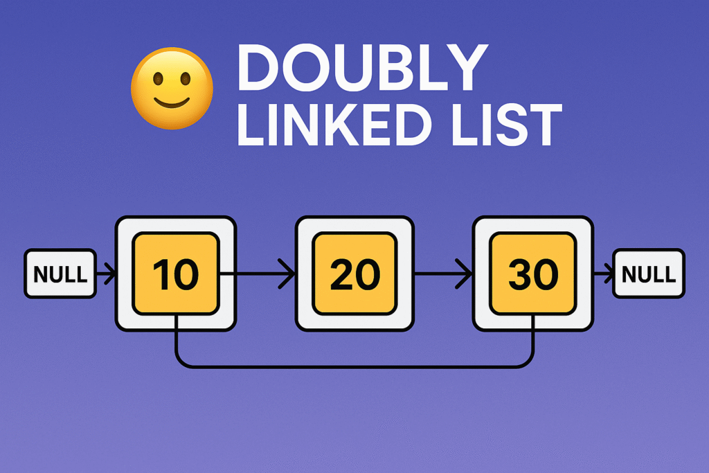
    Visual Representation of Doubly Linked List

    Let’s say we have 3 nodes with data: 10, 20, and 30.

    NULL <- [10] <-> [20] <-> [30] -> NULL
    

    Here:

    • Node 10’s prev is NULL
    • Node 20’s prev points to 10 and next to 30
    • Node 30’s next is NULL

    Basic Operations on Doubly Linked List

    1. Insertion

    • At the beginning
    • At the end
    • At a specific position

    2. Deletion

    • From the beginning
    • From the end
    • Specific node

    3. Traversal

    • Forward traversal (left to right)
    • Backward traversal (right to left)

    C Code Example: Basic DLL Operations

    #include <stdio.h>
    #include <stdlib.h>
    
    typedef struct Node {
        int data;
        struct Node* prev;
        struct Node* next;
    } Node;
    
    Node* head = NULL;
    
    // Insert at end
    void insertEnd(int value) {
        Node* newNode = (Node*)malloc(sizeof(Node));
        newNode->data = value;
        newNode->next = NULL;
    
        if (head == NULL) {
            newNode->prev = NULL;
            head = newNode;
            return;
        }
    
        Node* temp = head;
        while (temp->next != NULL)
            temp = temp->next;
    
        temp->next = newNode;
        newNode->prev = temp;
    }
    
    // Display forward
    void displayForward() {
        Node* temp = head;
        printf("DLL (forward): ");
        while (temp != NULL) {
            printf("%d <-> ", temp->data);
            temp = temp->next;
        }
        printf("NULL\n");
    }
    
    // Display backward
    void displayBackward() {
        Node* temp = head;
        if (!temp) return;
        
        // Go to last node
        while (temp->next != NULL)
            temp = temp->next;
    
        printf("DLL (backward): ");
        while (temp != NULL) {
            printf("%d <-> ", temp->data);
            temp = temp->prev;
        }
        printf("NULL\n");
    }
    
    int main() {
        insertEnd(10);
        insertEnd(20);
        insertEnd(30);
        
        displayForward();
        displayBackward();
        return 0;
    }
    

    Advantages of Doubly Linked List

    • Two-way traversal: You can navigate forward and backward.
    • Easier deletion: You can delete a node without needing the previous node pointer.
    • More flexible: Especially useful in complex data structures like Deques, Undo/Redo systems, Music Playlists, etc.

    Disadvantages of Doubly Linked List

    • More memory: Each node requires extra space for the prev pointer.
    • More complex: Handling pointers can be error-prone for beginners.

    Real-Life Applications of Doubly Linked List

    • Web browsers (backward and forward navigation)
    • Music playlist apps
    • Text editors (undo/redo operations)
    • Task managers (circular doubly linked lists for round-robin)

    Conclusion DLL

    Doubly Linked List
    Master Doubly Linked List in Data Structures (With Examples) 2025

    The Doubly Linked List is an essential topic in Data Structures and Algorithms (DSA). It offers a better way to manage dynamic data, especially when two-way traversal is needed. Though slightly more complex than a singly linked list, the benefits are powerful.

    Whether you’re preparing for a coding interview, building a system-level application, or just learning C programming, mastering DLLs will give you a strong foundation in memory management and pointer logic.

    FAQs of Doubly Linked List

    Q1: Is doubly linked list faster than singly linked list?
    Ans: DLL allows backward traversal and easier deletion, but it uses more memory. It’s more flexible, not necessarily faster.

    Q2: Where is DLL used in real life?
    Ans: Browser history, playlist navigation, undo/redo features, and memory management systems.

    Q3: What is the main drawback of doubly linked list?
    Ans: It uses extra memory due to the additional prev pointer and increases code complexity.

    Q4: How is a doubly linked list different from a circular doubly linked list?
    Ans: In a doubly linked list, the last node’s next pointer is NULL, whereas in a circular doubly linked list, the last node’s next points back to the head, forming a circle.

    Q5: Can a doubly linked list be empty?
    Ans: Yes, initially a doubly linked list can be empty with head pointing to NULL.

    Q6: How do you insert a node at the beginning of a doubly linked list?
    Ans: Create a new node, point its next to the current head, set the head’s prev to the new node, and then update head to the new node.

    Q7: What happens when you delete the last node in a doubly linked list?
    Ans: The second last node’s next pointer is set to NULL, and the last node is freed from memory.

    Q8: Is it possible to implement a stack using a doubly linked list?
    Ans: Yes, a doubly linked list can be used to implement a stack with push and pop operations.

    Q9: How does traversal in a doubly linked list work?
    Ans: You can traverse forward from head to NULL using next pointers or backward from the last node to head using prev pointers.

    Q10: What are the memory requirements for a doubly linked list node?
    Ans: Each node stores data plus two pointers (prev and next), so it uses more memory compared to a singly linked list node, which stores only one pointer.

    Q11: Can doubly linked lists have cycles? How to detect them?
    Ans: Yes, cycles can exist if nodes point back to earlier nodes. Cycle detection algorithms like Floyd’s Cycle-Finding Algorithm (tortoise and hare) can detect cycles.

    Q12: Are doubly linked lists used in databases?
    Ans: Yes, doubly linked lists are used to implement certain data structures like LRU caches, which are common in databases and operating systems.

    Q13: How do you reverse a doubly linked list?
    Ans: Swap the prev and next pointers for each node and update the head to the last node.

  • Linked List Explained: Master Complete Guide for Beginners 2026

    Introduction to Linked List

    If you’re learning Linked List data structures, you’ve probably come across the term Linked List. But what exactly is it? How does it work, and why do we even need it when we already have arrays?

    In this blog post, we’ll dive deep into linked list in data structure, understand how it differs from other data structures, explore the types of linked list, and learn about their practical advantages and use cases.

    What is a Linked List?

    A Linked List is a linear data structure where elements are stored in nodes, and each node points to the next one in the sequence. Unlike arrays, which store elements in contiguous memory locations, linked lists store data non-contiguously and use pointers to connect elements.

    Each node in a linked list contains:

    • Data (the value stored in the node)
    • Pointer (or reference) to the next node

    This unique structure makes linked lists highly flexible and efficient in certain scenarios.

    Why Use Linked List Instead of Arrays?

    Before diving into the types of linked list, let’s quickly understand why we’d choose a linked list over an array:

    ✅ Dynamic Size: Unlike arrays, linked lists don’t require specifying size in advance. Nodes can be added or removed without reallocating memory.

    ✅ Efficient Insertions/Deletions: Adding or removing elements doesn’t involve shifting elements, as in arrays.

    ✅ Memory Utilization: Useful when memory is fragmented or when the size of the dataset changes frequently.

    However, linked lists also have some disadvantages, like higher memory usage due to storing pointers and slower random access.

    Types of Linked List

    There are several types of linked list, each serving different use cases:

    1. Singly Linked List

    • Each node has a reference to the next node only.
    • Traversal is possible only in one direction.
    • Simple and widely used in basic implementations.

    Example:

    [10] → [20] → [30] → NULL
    

    2. Doubly Linked List

    • Each node has references to both next and previous nodes.
    • Allows traversal in both directions (forward and backward).
    • Slightly higher memory usage due to the extra pointer.

    Example:

    NULL ← [10] ↔ [20] ↔ [30] → NULL
    

    3. Circular Linked List

    • Last node points back to the first node, creating a circle.
    • Can be singly or doubly linked.
    • Useful in applications like round-robin scheduling.

    Example:

    [10] → [20] → [30] → [10] …
    

    Common Linked List Operations

    Understanding basic linked list operations is crucial. Let’s look at the most common:

    Insertion

    • Insert a new node at the beginning, middle, or end of the list.

    Deletion

    • Remove a node based on value or position.

    Traversal

    • Visit each node and perform an action (like printing values).

    Searching

    • Find whether a particular value exists in the linked list.

    Advantages of Linked List

    Let’s recap some advantages of linked list:

    • Dynamic memory allocation
    • No wasted memory (no predefined size)
    • Easier insertion/deletion
    • Useful for implementing stacks, queues, graphs, and more

    Applications of Linked List

    Here are some practical uses of linked list in data structure:

    • Implementing stacks and queues
    • Dynamic memory management
    • Browser history (back and forward functionality)
    • Undo/redo features in software
    • Hash table chaining

    Linked List vs Array: Quick Comparison

    FeatureArrayLinked List
    SizeFixedDynamic
    Memory AllocationContiguousNon-contiguous
    Insertion/DeletionCostly (shifting)Efficient
    Random AccessO(1)O(n)

    Conclusion

    A Linked List is a powerful and flexible data structure essential for any programmer’s toolkit. While it might seem complex initially, it offers significant advantages, especially when dealing with dynamic data and frequent insertions or deletions.

    Whether you’re preparing for coding interviews or simply expanding your programming knowledge, mastering linked list in data structure will give you a strong foundation for solving complex problems efficiently.

    Frequently Asked Questions (FAQ)

    Q1. What is a linked list in simple words?
    A linked list is a sequence of nodes where each node points to the next, making it easy to add or remove elements without shifting other data.

    Q2. Is linked list better than array?
    It depends. Linked lists are better for frequent insertions/deletions, but arrays are better for fast random access.

    Q3. What are the types of linked list?
    The main types include singly linked list, doubly linked list, and circular linked list.

    Q4. Where is linked list used in real life?
    Linked lists are used in browser history, memory management, music playlists, and many other applications.

  • Master pthreads tutorial | Beginner-Friendly Guide 2026

    pthreads tutorial explains pthreads (POSIX threads) in simple, beginner-friendly language. You’ll learn what threads are, why they’re useful, and how to create them using the pthread library in C. The article covers basic thread creation, joining, passing data between threads, and avoiding common issues like race conditions. It also includes example programs and common interview questions to help you feel confident using pthreads in real-world coding or interviews.

    What Are Threads?

    Imagine your computer running several tasks at once — like downloading a file, updating the screen, and playing music. Threads are the “mini-programs” inside a single process that let you do multiple tasks at the same time.

    • A process has its own memory space.
    • A thread shares memory space with other threads in the same process.

    Threads help programs:
    ✅ run faster on multi-core CPUs
    ✅ stay responsive (e.g. in apps with user interfaces)
    ✅ manage parallel tasks (e.g. computations, I/O)

    What is pthread?

    pthreads (POSIX threads) is a library in C/C++ on Unix-like systems (Linux, macOS, etc.) that helps you create and manage threads.

    • Defined in pthread.h
    • Functions start with pthread_

    How to Create a Thread

    Here’s the simplest pthread program:

    #include <stdio.h>
    #include <pthread.h>
    
    void* myThreadFunction(void* arg) {
        printf("Hello from the new thread!\n");
        return NULL;
    }
    
    int main() {
        pthread_t threadId;
        
        // Create a new thread
        pthread_create(&threadId, NULL, myThreadFunction, NULL);
    
        // Wait for the thread to finish
        pthread_join(threadId, NULL);
    
        printf("Back in main thread.\n");
        return 0;
    }
    

    How this works:

    ✅ pthread_create(...) creates a thread and runs myThreadFunction in it.

    ✅ pthread_join(...) waits until the thread finishes.

    pthread_create – Function Details

    int pthread_create(
        pthread_t *thread,          // Thread ID output
        const pthread_attr_t *attr, // Attributes (can be NULL)
        void *(*start_routine)(void *), // Function the thread runs
        void *arg                   // Argument passed to that function
    );
    

    Example:

    pthread_create(&threadId, NULL, myThreadFunction, NULL);
    

    Once a thread starts, the main thread might finish too early. We don’t want the program to exit while other threads are still running. So, we join the thread:

    pthread_join(threadId, NULL);
    

    This waits until the thread is done.

    Passing Data to Threads

    Threads often need data. You can pass arguments via the void* argument:

    #include <stdio.h>
    #include <pthread.h>
    
    void* printNumber(void* arg) {
        int num = *(int*)arg;
        printf("Thread received number: %d\n", num);
        return NULL;
    }
    
    int main() {
        pthread_t tid;
        int val = 42;
        pthread_create(&tid, NULL, printNumber, &val);
        pthread_join(tid, NULL);
        return 0;
    }
    

    Threads Share Memory!

    Unlike processes, threads share global variables and heap memory.

    Synchronization with Mutexes

    Mutex = Mutual Exclusion. It prevents simultaneous access.

    Example:

    #include <stdio.h>
    #include <pthread.h>
    
    pthread_mutex_t lock;
    
    void* myThread(void* arg) {
        pthread_mutex_lock(&lock);
        // Critical section
        printf("Thread in critical section\n");
        pthread_mutex_unlock(&lock);
        return NULL;
    }
    
    int main() {
        pthread_t tid;
        pthread_mutex_init(&lock, NULL);
        
        pthread_create(&tid, NULL, myThread, NULL);
        pthread_join(tid, NULL);
        
        pthread_mutex_destroy(&lock);
        return 0;
    }
    
    FunctionDescription
    pthread_exit()End a thread voluntarily
    pthread_self()Get the current thread ID
    pthread_mutex_init()Initialize a mutex
    pthread_mutex_lock()Lock a mutex
    pthread_mutex_unlock()Unlock a mutex
    pthread_mutex_destroy()Free mutex resources

    Advantages of pthreads

    ✅ Speed — threads can run concurrently.
    ✅ Shared memory — no need for complex communication like pipes or sockets.
    ✅ Lightweight — creating threads costs less than creating processes.

    pthread Interview Questions

    Here are some beginner-to-intermediate interview questions on pthreads:

    Q1. What is the difference between a process and a thread?

    • Process: Separate memory space, separate code, own resources.
    • Thread: Shares memory and resources with other threads in same process.

    Q2. What is pthread?

    A POSIX standard library in C/C++ for creating and managing threads on Unix-like systems.

    Q3. How do you create a thread using pthread?

    Using pthread_create:

    pthread_create(&tid, NULL, myThreadFunction, NULL);
    

    Q4. How can you wait for a thread to finish?

    By calling:

    pthread_join(threadId, NULL);
    

    Q5. Why do we need synchronization primitives like mutexes?

    Because threads share memory. To avoid race conditions when two threads access or modify the same data]\\][]\

    Q6. What is a race condition?

    When two or more threads read or write shared data at the same time, leading to unpredictable results.

    Q7. What’s the purpose of pthread_mutex_lock and pthread_mutex_unlock?

    They lock/unlock a mutex so that only one thread can enter a critical section at a time.

    Q8. Can you pass arguments to threads in pthread?

    Yes! Use the void* arg parameter in pthread_create to pass data.

    Q9. What happens if you don’t call pthread_join?

    The main thread might exit before other threads finish. This may terminate the whole process before threads complete their work.

    Q10. What is a deadlock?

    When two or more threads each hold a lock and wait forever for each other to release it.

    How to Avoid Race Conditions

    What is a Race Condition?

    A race condition happens when:

    • Two or more threads access the same variable or data at the same time
    • At least one of them writes to it

    Result: The outcome depends on who “wins the race” — i.e. which thread runs first. This causes bugs that happen randomly.

    Example of a race condition:

    #include <stdio.h>
    #include <pthread.h>
    
    int counter = 0;
    
    void* increment(void* arg) {
        for (int i = 0; i < 100000; i++) {
            counter++;
        }
        return NULL;
    }
    
    int main() {
        pthread_t t1, t2;
        pthread_create(&t1, NULL, increment, NULL);
        pthread_create(&t2, NULL, increment, NULL);
        
        pthread_join(t1, NULL);
        pthread_join(t2, NULL);
        
        printf("Final counter value: %d\n", counter);
        return 0;
    }
    

    Expected output: 200000
    Actual output: Sometimes less than 200000!

    How to Avoid Race Conditions

    Here’s how you can avoid race conditions in pthreads:

    ✅ 1. Use Mutexes

    A mutex lets only one thread enter a critical section at a time.

    Example:

    #include <stdio.h>
    #include <pthread.h>
    
    int counter = 0;
    pthread_mutex_t lock;
    
    void* increment(void* arg) {
        for (int i = 0; i < 100000; i++) {
            pthread_mutex_lock(&lock);
            counter++;
            pthread_mutex_unlock(&lock);
        }
        return NULL;
    }
    
    int main() {
        pthread_t t1, t2;
        pthread_mutex_init(&lock, NULL);
    
        pthread_create(&t1, NULL, increment, NULL);
        pthread_create(&t2, NULL, increment, NULL);
    
        pthread_join(t1, NULL);
        pthread_join(t2, NULL);
    
        pthread_mutex_destroy(&lock);
        
        printf("Final counter value: %d\n", counter);
        return 0;
    }
    

    Now, output is reliably 200000.

    ✅ 2. Use Read-Write Locks

    If many threads read and only some write, use read-write locks (pthread_rwlock).

    • Multiple readers allowed.
    • Writers get exclusive access.

    ✅ 3. Use Atomic Operations

    For simple variables, you can use atomic operations instead of mutexes.

    Example (using GCC atomic built-ins):

    __sync_fetch_and_add(&counter, 1);
    

    These are lock-free and faster.

    ✅ 4. Minimize Shared Data

    • Avoid sharing data between threads if you can.
    • Give each thread its own variables.
    • Less sharing → fewer race conditions!

    ✅ 5. Proper Thread Join / Synchronization

    Always join threads before accessing shared results.

    pthread_join(t1, NULL);
    pthread_join(t2, NULL);
    

    Otherwise, main might read data while threads are still changing it.

    ✅ 6. Condition Variables (Advanced)

    When threads wait for some condition to become true, combine mutexes with condition variables for safe signaling.

    Simple Rule

    “Protect all shared data with synchronization.”

    Any time multiple threads:

    • Read and write shared variables
    • Modify global variables
    • Update shared structures

    → Use mutexes or other mechanisms.

    How To Spot Race Conditions?

    They often show up as:

    • Random crashes
    • Wrong calculation results
    • Bugs that “sometimes” happen

    FAQ – Beginner-Friendly Guide: Understanding pthreads

    Q1. What are pthreads?

    Answer:
    pthreads stands for POSIX threads. It’s a library in C/C++ used to create and manage threads on Unix-like systems like Linux and macOS.

    Q2. Why should I use threads?

    Answer:
    Threads help your program do multiple things at once, like:

    • Handling many tasks faster
    • Keeping apps responsive
    • Using multi-core CPUs efficiently

    Q3. What’s the difference between a process and a thread?

    Answer:

    • A process has its own memory space.
    • A thread shares memory with other threads in the same process.

    Threads are lighter and faster to create than processes.

    Q4. How do I create a thread in pthread?

    Answer:
    Use pthread_create. Example:

    pthread_create(&threadId, NULL, myFunction, NULL);

    Q5. What is pthread_join?

    Answer:
    pthread_join waits for a thread to finish before moving on. It prevents your program from ending too soon while threads are still working.

    Q6. Can I pass data to threads?

    Answer:
    Yes! You can pass a pointer as an argument to your thread function.

    Example:

    pthread_create(&tid, NULL, myFunction, &myData);
    

    Q7. What is a race condition?

    Answer:
    A race condition happens when two threads change the same data at the same time, causing unpredictable results.

    Q8. How do I avoid race conditions in pthreads?

    Answer:
    Use a mutex to lock shared data so only one thread can change it at a time.

    Q9. Do threads share variables?

    Answer:
    Yes. Threads share:

    • Global variables
    • Heap memory

    Each thread has its own stack for local variables.

    Q10. Is pthread available on Windows?

    Answer:
    pthreads is mainly for Unix-like systems. On Windows, you might use:

    • Windows Threads API
    • Libraries like pthreads-win32
    • C++11’s <thread> instead

    Tutorials & Guides

    1. Multithreaded Programming (POSIX pthreads Tutorial) – randu.org
      A comprehensive guide covering thread synchronization, mutexes, and practical examples to get you started with pthreads.
    2. Multi-Threaded Programming With POSIX Threads – Villanova University
      A well-structured tutorial introducing POSIX threads, including examples and explanations suitable for beginners.
    3. POSIX Threads Programming – LLNL HPC Tutorials
      A detailed guide from Lawrence Livermore National Laboratory, covering thread creation, synchronization, and more.

    🎥 Video Tutorials

    📚 Reference Materials

  • Single Number LeetCode Solution C++ | Master XOR Trick | Leetcode Solution (2026)

    Single Number LeetCode Solution C++ : Learn the most efficient way to solve the Single Number problem on LeetCode using C++ and the XOR bitwise operator. Understand time complexity, code explanation, and why this approach works.

    Introduction of Single Number LeetCode Solution C++

    Looking for an efficient Single Number LeetCode Solution in C++? You’re in the right place!

    The Single Number problem is one of the most popular coding interview questions on platforms like LeetCode and helps test your understanding of bit manipulation.

    Let’s dive in and see how you can solve it in linear time and constant space.

    Problem Statement: Single Number

    LeetCode 136. Single Number

    Given a non-empty array of integers nums, every element appears twice except for one. Find that single one.

    You must implement a solution with a linear runtime complexity and use only constant extra space.

    Example:

    Input: nums = [4,1,2,1,2]
    Output: 4
    

    How to Solve the Single Number Problem

    At first glance, you might think of using:

    • Hash maps to count occurrences
    • Sorting the array and checking neighbors

    But both use extra space or more than O(n) time.

    Instead, there’s a beautiful trick using the XOR bitwise operator.

    Fantastic — let’s structure your blog to show progressive solutions to the Single Number problem:

    ✅ Brute-force solution (simplest but inefficient)
    ✅ Better (scalable) solution (using a map or set)
    ✅ Perfect solution (optimal XOR trick)

    1. Brute Force Solution (O(n²))

    Approach

    • For each number, count how many times it appears in the array.
    • Return the one that appears only once.

    Code

    class Solution {
    public:
        int singleNumber(vector<int>& nums) {
            int n = nums.size();
            for (int i = 0; i < n; i++) {
                int count = 0;
                for (int j = 0; j < n; j++) {
                    if (nums[i] == nums[j]) {
                        count++;
                    }
                }
                if (count == 1) {
                    return nums[i];
                }
            }
            return -1; // No single number found
        }
    };
    

    Complexity

    • Time: O(n²)
    • Space: O(1)

    ✅ Easy to understand
    ❌ Slow for large arrays

    2. Better Solution Using Hash Map (O(n))

    Approach

    • Use a hash map to count frequencies.
    • Return the number whose frequency is 1.

    Code

    class Solution {
    public:
        int singleNumber(vector<int>& nums) {
            unordered_map<int, int> freq;
            for (int num : nums) {
                freq[num]++;
            }
            for (auto& pair : freq) {
                if (pair.second == 1) {
                    return pair.first;
                }
            }
            return -1;
        }
    };
    

    Complexity

    • Time: O(n)
    • Space: O(n)

    ✅ Linear time
    ❌ Extra space required

    3. Perfect Solution Using XOR (O(n), O(1))

    Recall these properties of XOR (^):

    • a ^ a = 0 (a number XOR itself is zero)
    • a ^ 0 = a
    • XOR is commutative and associative (order doesn’t matter)

    So if every number appears twice, XOR-ing all numbers cancels out the pairs:

    a ^ a ^ b = 0 ^ b = b
    

    Hence, the Single Number remains after XOR-ing all numbers.

    C++ Code – Single Number LeetCode Solution

    Here’s the optimized solution in C++ that you provided:

    class Solution {
    public:
        int singleNumber(vector<int>& nums) {
    
            int result = 0;
            for (int num : nums) {
                result ^= num;
            }
            return result;
        }
    };
    

    Step-by-Step Code Explanation

    Let’s break it down line by line.

    Line 1

    class Solution {
    

    Defines a class named Solution as required by LeetCode’s online judge.

    Line 2

    public:
    

    Marks methods as accessible outside the class.

    Line 3

    int singleNumber(vector<int>& nums) {
    
    • Defines a function singleNumber
    • Takes a reference to a vector of integers nums
    • Returns an int

    Line 4

    int result = 0;
    
    • Initialize result to 0.
    • This variable will hold the XOR of all numbers.

    Line 5

    for (int num : nums) {
        result ^= num;
    }
    
    • Loops through each integer in the array nums.
    • XORs it with result.
    • Duplicate numbers cancel each other out.
    • Only the single number remains.

    Example trace for [4,1,2,1,2]:

    0 ^ 4 = 4
    4 ^ 1 = 5
    5 ^ 2 = 7
    7 ^ 1 = 6
    6 ^ 2 = 4
    

    So the single number is 4.

    Line 8

    return result;
    

    Returns the unique number found.

    Time and Space Complexity

    ✅ Time Complexity: O(n)
    ✅ Space Complexity: O(1)

    This solution is optimal and easily fits the problem’s constraints.

    Summary

    SolutionTimeSpace
    Brute ForceO(n²)O(1)
    Hash MapO(n)O(n)
    XOR (Optimal)O(n)O(1)

    Python Solution

    Focus Keyword: Single Number LeetCode Solution Python

    class Solution:
        def singleNumber(self, nums):
            result = 0
            for num in nums:
                result ^= num
            return result
    

    Explanation:

    • Initialize result = 0.
    • XOR each element into result.
    • Pairs cancel out; single number remains.

    ✅ Time Complexity: O(n)
    ✅ Space Complexity: O(1)

    Java Solution

    Focus Keyword: Single Number LeetCode Solution Java

    class Solution {
        public int singleNumber(int[] nums) {
            int result = 0;
            for (int num : nums) {
                result ^= num;
            }
            return result;
        }
    }
    

    Explanation:

    • result starts at 0.
    • For each num in array, XOR it with result.
    • The unique number remains after all XORs.

    ✅ Time Complexity: O(n)
    ✅ Space Complexity: O(1)

    JavaScript Solution

    Focus Keyword: Single Number LeetCode Solution JavaScript

    var singleNumber = function(nums) {
        let result = 0;
        for (let num of nums) {
            result ^= num;
        }
        return result;
    };
    

    Explanation:

    • result initialized as 0.
    • Loop through nums.
    • XOR all numbers together.
    • Duplicate numbers cancel out, leaving the single number.

    ✅ Time Complexity: O(n)
    ✅ Space Complexity: O(1)

    Advantages of XOR Approach

    • No extra data structures required
    • Runs in linear time
    • Simple and elegant logic

    If you’re preparing for coding interviews, knowing this XOR trick can save you crucial time!

    🔗 Related LeetCode Problems

    Conclusion

    The XOR trick is a brilliant way to solve the Single Number problem efficiently in C++. Understanding how XOR cancels out duplicate numbers is essential for solving similar problems in coding interviews.

    FAQ – Single Number LeetCode Solution

    Q1. What is the Single Number problem on LeetCode?

    The Single Number problem on LeetCode asks you to find the only integer in an array that appears exactly once, while all other integers appear twice. You must solve it in linear time and with constant space complexity.

    Q2. How does the XOR trick help solve the Single Number problem?

    The XOR operator cancels out identical numbers because a ^ a = 0. When you XOR all numbers in the array, duplicates cancel each other, leaving only the unique number behind.

    Q3. What is the time complexity of the XOR solution for Single Number?

    The XOR solution runs in O(n) time, where n is the number of elements in the array.

    Q4. What is the space complexity of the XOR solution for Single Number?

    It uses O(1) space because you only store a single integer result, regardless of the input size.

    Q5. Can the Single Number problem be solved without bit manipulation?

    Yes, but less efficiently. You could use a hash map to count occurrences or sort the array and check neighbors. However, these methods either use extra space or exceed O(n) time complexity.

    Q6. Can the Single Number problem be solved in Python, Java, or JavaScript?

    Absolutely! The same XOR logic works in Python, Java, C++, JavaScript, and many other languages. It’s language-agnostic because XOR is a universal bitwise operation.

    Q7. Is the XOR method safe for negative numbers?

    Yes! XOR works on the bit-level representation of integers, so it handles negative numbers correctly.

    Q8. What LeetCode problems are similar to Single Number?

    • Single Number II (LeetCode 137) – Find the number appearing only once when every other appears three times.
    • Single Number III (LeetCode 260) – Find two numbers appearing once when every other appears twice.

    Q9. Why can’t I just sort the array to solve Single Number?

    While sorting works, it’s O(n log n) time, which doesn’t meet the problem’s linear time requirement. The XOR method is faster and uses constant space.

    Q10. Is Single Number a common coding interview question?

    Yes! The Single Number problem is frequently asked in coding interviews because it tests knowledge of bit manipulation, time complexity, and space optimization.

  • Next-Gen Test and Measurement Tools Drive High-Frequency, Multi-Domain Innovations (2026)

    As modern electronics continue pushing boundaries in speed and complexity, engineers face growing challenges in testing high-frequency and multi-domain systems. To meet these demands, leading players in the test and measurement industry are unveiling advanced solutions designed to address signal integrity, timing accuracy, and RF performance in one unified platform.

    The Rise of Multi-Domain Systems in 2025

    From 5G and Wi-Fi 7 to advanced radar and satellite communication systems, today’s technologies often involve multiple domains—digital, analog, RF, and optical—working together in real-time. As a result, traditional test methods are no longer sufficient. Engineers now require tools capable of synchronously analyzing multiple signal types across various time and frequency domains.

    What’s New in Test & Measurement?

    Recently, major T&M companies introduced solutions that offer unprecedented bandwidth, sampling rate, and resolution. These include:

    • High-Bandwidth Oscilloscopes with bandwidths exceeding 100 GHz, ideal for capturing ultra-fast transitions and jitter.
    • Mixed-Signal Analyzers capable of cross-domain correlation between RF and digital logic.
    • Real-Time Spectrum Analyzers featuring enhanced dynamic range and time-correlated capture.
    • Vector Network Analyzers (VNAs) designed for characterizing high-frequency passive and active components with precision.

    These tools are not just faster—they’re smarter. Many come equipped with AI-enhanced analysis, automated calibration, and intuitive user interfaces for faster setup and measurement accuracy.

    Why It Matters: Key Benefits

    • Improved Signal Integrity Testing: High-speed digital designs rely on accurate jitter, skew, and eye diagram measurements—now achievable with real-time correlation tools.
    • Faster Time-to-Market: Integrated platforms reduce the need for separate test equipment, speeding up the validation process.
    • Multi-Domain Insight: Engineers can visualize and debug interactions across RF, analog, and digital domains in one interface.
    • Enhanced 5G and mmWave Testing: With support for higher frequencies, these solutions ensure devices are compliant with the latest standards.

    Applications Driving the Demand

    • 5G/6G Communication Systems
    • Aerospace & Defense Radar
    • Automotive mmWave Sensors (ADAS)
    • Quantum Computing & Research
    • High-Speed Serial Interfaces (PCIe, USB4, DDR5)

    Future Outlook: Converging Domains, Unified Tools

    Looking forward, as domains continue to converge, test and measurement tools will evolve to become more integrated, cloud-connected, and software-defined. Test automation, AI-based diagnostics, and digital twin simulations are likely to redefine how hardware is validated in real-time.

  • Nordic Semiconductor Unveils Advanced Power Management IC for Miniature Battery Devices

    Nordic Semiconductor nPM1304

    Nordic Semiconductor has launched the nPM1304, an ultra-low power power management IC (PMIC) designed specifically for compact, battery-operated devices. This advanced PMIC offers precise voltage regulation, efficient USB-C input support, and an innovative model-based fuel gauging system that accurately monitors battery state of charge while minimizing power consumption. Ideal for next-generation wearables and sensor applications, the nPM1304 delivers comprehensive battery management and system-level features, making it a perfect solution for miniaturized electronics demanding both power efficiency and reliability.

    Nordic Semiconductor Unveils Advanced Power Management IC for Miniature Battery Devices
    Nordic Semiconductor has unveiled its latest power management integrated circuit (PMIC), specifically engineered for compact electronic devices powered by small-capacity batteries. The new PMIC, named nPM1304, builds on the success of its predecessor, the nPM1300, and offers advanced power efficiency tailored for next-generation wearable technology and sensor applications.

    Next-Generation PMIC Designed for Miniaturized Battery-Powered Devices

    The nPM1304 power management IC is designed to meet the growing demand for compact and energy-efficient solutions in the wearables and IoT market. It delivers four independently controlled power rails via two 200mA buck regulators and two 100mA load switches (which can also be configured as 50mA LDOs). Each power rail offers precise voltage regulation from 1.0 V up to 3.3 V, enabling versatile application support.

    Supporting USB-C input, the nPM1304 includes an integrated input regulator capable of handling 4.0 V to 5.5 V with a 1.5 A current limit and tolerates transient voltages up to 22 V, making it highly adaptable to varying power sources.

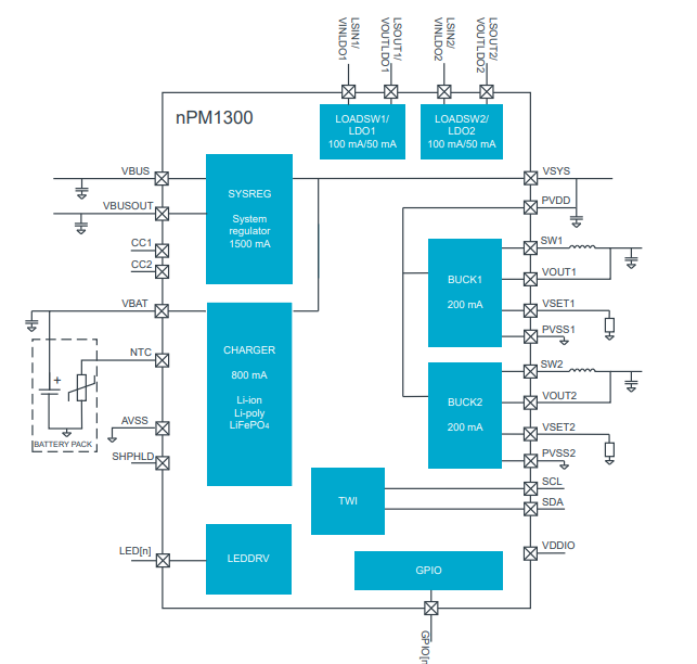
    [ VBUS ] ──► [ SYSREG ]
                      │
                      ▼
                   VSYS
                      │
     ┌────────────────┴─────────────┐
     │                              │
     │                              │
     │                          [ CHARGER ]
     │                              │
     │                   +----------+----------+
     │                   │                     │
     │                [ Battery ]         [ NTC ]
     │                                         │
     │                                    [ SHPHLD ]
     │                                         │
     │                                [ LEDDRV ]
     │
     │
     ▼
    [ BUCK1 ] ──► VOUT1
       │
     [ VSET1 ]
    
    [ BUCK2 ] ──► VOUT2
       │
     [ VSET2 ]
    
    [ LDO1 / LOADSW1 ] ──► LDO1_VOUT
    [ LDO2 / LOADSW2 ] ──► LDO2_VOUT
    
    [ GPIO ]
    [ TWI (I2C) ]
       │
    [SCL]  [SDA]
    

    Innovative Model-Based Fuel Gauging for Accurate Battery Monitoring

    One of the standout features of the nPM1304 PMIC is its model-based fuel gauging system. Unlike traditional coulomb counting methods that require continuous power consumption and recalibration, Nordic’s approach estimates the battery state of charge by analyzing voltage, current, and temperature data. This results in highly accurate battery monitoring with significantly reduced power consumption — drawing just 8 µA during active operation and zero current in sleep mode. This ultra-low power design is especially beneficial for devices with stringent energy budgets.

    Nordic Semiconductor Unveils Advanced Power Management IC for Miniature Battery Devices

    Comprehensive Battery Management with Programmable Charging

    The device supports a linear battery charger compatible with multiple chemistries, including Li-ion, Li-polymer, and LiFePO₄. Programmable charge currents range from 4 mA to 100 mA, and the termination voltage is adjustable between 3.5 V and 4.65 V, enabling flexible charging profiles tailored to specific battery types.

    Additional system-level features include watchdog and boot timers, power loss warning, configurable hard reset functions, recovery from failed boots, and a user-friendly I²C interface for system configuration. Developers also benefit from five general-purpose I/Os and three LED drivers integrated within the chip.

    Why Model-Based Fuel Gauging Outperforms Traditional Coulomb Counting

    Traditional coulomb counting estimates battery charge by measuring the current flowing in and out of the battery using sense resistors and integrating the results over time. Although effective, this method is prone to cumulative errors and requires periodic recalibration, which can be impractical for small devices with low and irregular current draws.

    Moreover, coulomb counting circuitry demands continuous power, often consuming a notable fraction of the device’s limited energy budget. Nordic’s model-based fuel gauge sidesteps these issues by employing a dynamic battery model that efficiently interprets sensor data, reducing energy use while maintaining state-of-charge accuracy.

    Nordic Semiconductor Unveils Advanced Power Management IC for Miniature Battery Devices

    Meeting Industry Demands for Compact and Efficient Power Management

    The nPM1304 addresses the growing need for compact, ultra-efficient power management ICs that support the increasing miniaturization of wearable and sensor devices. Nordic Semiconductor is now offering samples of this PMIC to developers looking to optimize power consumption in their battery-operated embedded systems.

    Advantages of nPM1300 PMIC

    ✅ Highly Integrated Solution

    • Combines charger, regulators, LED drivers, and GPIO in a single chip → reduces PCB space and BOM cost.

    ✅ Battery Charger Included

    • Supports Li-ion, Li-poly, and LiFePO4 batteries.
    • Integrated battery charging (up to 800 mA) eliminates need for separate charger ICs.

    ✅ Low Power Consumption

    • Suitable for battery-operated designs.
    • System regulator (SYSREG) and low quiescent current help extend battery life.

    ✅ Multiple Outputs

    • Two buck converters and two LDOs/Load switches allow powering different rails with separate voltages.
    • Flexible for different peripherals (MCU, sensors, radios).

    ✅ I²C Interface (TWI)

    • Programmable control of output voltages and other parameters → dynamic power management.
    • Enables MCU or SoC to adjust power rails in software.

    ✅ Integrated LED Drivers

    • Useful for status indicators or backlighting without extra driver ICs.

    ✅ Compact Solution

    • Smaller PCB footprint ideal for wearable, IoT, and portable devices.

    Disadvantages of nPM1300 PMIC

    ❌ Current Limitations

    • Buck converters limited to 200 mA → insufficient for high-power loads like large displays or motors.
    • LDO/Load switches limited to 100 mA / 50 mA.

    ❌ Complexity in Configuration

    • Requires software configuration via TWI → not purely hardware plug-and-play.
    • Might add development time for tuning voltages and power sequences.

    ❌ Limited Battery Chemistries

    • Although supporting common battery types, not suitable for NiMH, NiCd, or other less-common chemistries.

    ❌ Cost

    • Integrated PMICs can be more expensive than discrete solutions in ultra-low-cost designs.

    Real-Time Applications

    The nPM1300 is perfect for low-power embedded and portable applications requiring power efficiency and small form factor. Real-time examples:

    ✅ Wearable Devices

    • Smartwatches
    • Fitness bands
    • Medical patches

    ✅ IoT Devices

    • Wireless sensors
    • Smart home devices
    • Asset tracking tags

    ✅ Portable Medical Devices

    • Glucose monitors
    • Portable ECG devices

    ✅ Wireless Audio

    • Earbuds
    • Bluetooth headsets

    ✅ Compact Industrial Devices

    • Portable measurement tools
    • Handheld scanners

    ✅ Remote Controls / Smart Tags

    • Low-power BLE or proprietary RF remotes
    • RFID/NFC-enabled tags
  • AI Hardware in 2026: Master How Memory Architecture Is Defining System Design


    AI Hardware : Discover how booming AI workloads drive skyrocketing memory demands, challenging hardware design, supply chains, and BOM management. Learn how engineers are navigating AI memory architectures, sourcing risks, and performance trade-offs.

    Artificial intelligence (AI) is transforming everything—from smart wearables and voice assistants to autonomous vehicles and massive cloud-scale models. But beneath the headlines about powerful GPUs and lightning-fast accelerators lies a critical piece of the puzzle: memory.

    As AI applications explode in size and complexity, memory has emerged as a major bottleneck in modern hardware design. Whether you’re training a generative model in a datacenter or running real-time object detection on an edge device, memory capacity and bandwidth now dictate your system’s performance, power efficiency, and thermal stability.

    Why AI Workloads Demand More—and Faster—Memory

    AI workloads are inherently data-hungry. Deep learning models rely on rapid access to large datasets, model weights, and intermediate computations. As models grow in scale, traditional memory solutions can no longer keep up.

    To meet these demands, hardware designers are adopting specialized memory architectures, including:

    • High-Bandwidth Memory (HBM): Delivers massive I/O and throughput for AI training workloads.
    • GDDR6 / GDDR7: Ideal for graphics-intensive and inference-heavy tasks.
    • LPDDR5 / LPDDR5X: Balances performance and power for edge AI devices.
    • 3D-Stacked DRAM: Increases capacity while minimizing physical footprint.
    • Emerging Non-Volatile Memories (MRAM, ReRAM): Useful for persistent AI states and faster edge boot times.

    However, each of these technologies introduces unique design challenges around power, thermal management, and system integration.

    Why Memory-First Hardware Design Is Essential

    Traditional hardware design often focused on selecting processors first and then fitting memory accordingly. Today, AI system architects are adopting a memory-first approach. This strategy starts with evaluating:

    • Required memory capacity to store vast AI models and datasets
    • Necessary memory bandwidth to avoid data bottlenecks
    • Power consumption targets, especially for edge AI devices
    • Thermal design implications of memory types like 3D-stacked DRAM
    • Component availability amid ongoing supply chain challenges

    Starting hardware design with memory considerations ensures that AI solutions achieve optimal performance and reliability.

    Exploring Memory Technologies for AI Applications

    AI hardware designers must carefully select from a variety of memory technologies, each with its own advantages and trade-offs:

    • High-Bandwidth Memory (HBM): Offers exceptional data throughput via 3D stacking, ideal for high-performance AI training and inference in data centers, though with increased cost and thermal management needs.
    • GDDR6 and GDDR7: Widely used in GPUs, providing strong performance at a reasonable price point.
    • LPDDR5 and LPDDR5X: Energy-efficient choices suited for mobile and edge AI applications where power is limited.
    • Emerging non-volatile memories such as MRAM and ReRAM promise faster speeds and lower power but are still emerging in AI hardware markets.

    Addressing PCB Design and EMI Complexities

    Integrating advanced memory into AI hardware introduces several engineering challenges:

    • High-speed memory demands intricate PCB routing and signal integrity management.
    • Elevated data rates increase susceptibility to electromagnetic interference (EMI), requiring careful layout and shielding.
    • Thermal constraints from dense memory packages necessitate innovative cooling solutions.

    Successfully overcoming these issues is crucial for maintaining system stability and performance.

    Overcoming Supply Chain and BOM Challenges

    The global semiconductor supply chain remains unpredictable, with memory components among the most affected. AI hardware teams must implement robust Bill of Materials (BOM) management to:

    • Monitor component lead times and potential shortages
    • Identify alternative memory parts early to avoid project delays
    • Balance cost and availability to meet project budgets

    Effective BOM management is vital for timely AI hardware delivery.

    Special Considerations for Edge AI Memory

    Edge AI devices present unique challenges where memory must balance performance, power efficiency, and size. Edge deployments require:

    • Low-power memory such as LPDDR5X to extend battery life
    • Compact designs to fit in constrained physical spaces
    • Rigorous thermal design to prevent overheating without bulky cooling

    This makes memory selection and hardware design a critical, nuanced task for edge AI solutions.

    AI Hardware in 2025 Master How Memory Architecture Is Defining System Design
    AI Hardware in 2025 Master How Memory Architecture Is Defining System Design

    Memory Selection Now Drives Hardware Design Decisions

    Traditionally, engineers picked CPUs or GPUs first, then sorted out the memory. But in the AI era, that paradigm has flipped. Memory selection often dictates the entire hardware architecture.

    Consider these trade-offs:

    • GDDR6 offers high bandwidth for fast AI inference—but requires complex PCB routing, dedicated power rails, and careful thermal design.
    • LPDDR5 conserves battery life in mobile or edge devices—but comes with bandwidth limitations that can restrict model size or processing speed.
    • HBM enables tremendous throughput for AI training—but demands advanced packaging and innovative cooling solutions like vapor chambers or liquid cooling, significantly impacting cost.

    Moreover, AI projects often lock in memory choices early, before software models and firmware are fully stable. A misstep can lead to costly board redesigns or limit future upgrades.

    PCB layout and 3D visualization tools, such as Altium’s platform, are invaluable for anticipating how memory choices affect placement, routing complexity, and thermal strategies.

    Navigating Volatility in the AI Memory Supply Chain

    The AI boom has turned memory components—especially DRAM and NAND—into strategic assets. Yet the global memory supply chain remains volatile and geographically concentrated:

    • South Korea dominates DRAM production.
    • Taiwan leads advanced packaging and foundry services.
    • Japan supplies critical materials and specialty memory.

    This concentration introduces significant risks, including:

    • Geopolitical instability (e.g., tensions in the Taiwan Strait).
    • Export restrictions and trade barriers.
    • Bottlenecks in EUV lithography and specialized DRAM manufacturing.
    • Material shortages (e.g., fluorinated gases, specialty photoresists).

    For engineers building AI-enabled products, these factors mean longer lead times, unpredictable costs, and increased risk of component obsolescence.

    BOM (Bill of Materials) management tools, like Altium 365, empower hardware teams to quickly identify, source, and secure memory components early in the design process. This proactive approach is critical for mitigating supply chain disruptions and avoiding costly project delays.

    It’s Not Just About More Memory—It’s About Smarter Memory Access

    In AI hardware, simply adding more memory isn’t enough. What matters is having the right type of memory, in the right place, connected in the right way.

    Modern AI architectures demand careful planning around:

    • Tightly Coupled Memory: Reduces latency but requires deep integration with processors or SoCs.
    • Loosely Coupled Memory: Offers flexibility but can introduce bandwidth bottlenecks.
    • Memory Access Patterns: Optimizations like tensor reuse, strided access, or sparsity improve performance and power efficiency.
    • Partitioning Strategies: Storing different data types—weights, activations, intermediate results—in separate memory tiers (e.g., HBM, LPDDR, NVM) can dramatically influence speed, thermal behavior, and battery life.

    Compatibility is another critical hurdle. Engineers must ensure that chosen memory technologies are electrically and logically compatible with AI chips, FPGAs, and SoCs. A mismatch can cause performance bottlenecks, excessive power consumption, or wasted investments in high-performance compute hardware.

    Memory Strategy Is Now a Competitive Advantage

    Companies succeeding in AI hardware aren’t just focused on raw performance—they’re building resilience into their memory strategies from day one.

    Winning teams:

    • Analyze sourcing risks and part lifecycles during memory selection.
    • Simulate memory access and throughput early in the design process.
    • Foster cross-functional collaboration between hardware, software, and supply chain teams.
    • Leverage modern design platforms for real-time collaboration and component intelligence.

    When hardware and sourcing teams operate in silos, decisions around memory are delayed or made in isolation, leading to costly redesigns or missed product launch windows. Integrated collaboration ensures teams can identify alternatives, navigate shortages, and build systems that balance performance, power efficiency, and supply chain security.As AI models grow exponentially, hardware designers face a pressing need to prioritize memory solutions that match the computational surge. From data centers harnessing HBM to edge devices leveraging LPDDR5X, understanding the trade-offs in memory capacity, bandwidth, power, and supply is essential.

    Only by embracing a memory-first hardware design philosophy, coupled with strategic BOM management and advanced PCB engineering, can hardware teams build AI platforms that truly keep pace with the exploding demand for memory in 2025 and beyond.

    Memory has become the new battleground in the race to deliver innovative AI products. Designers who treat memory not as an afterthought—but as a core architectural priority—will lead the way in the AI revolution.

    You can also Visit other tutorials of Embedded Prep 

    Special thanks to @mr-raj for contributing to this article on Embedded Prep

  • CAN Interview Questions : Master Beginner-Friendly Tutorial [2026]

    CAN Interview Questions : Are you preparing for a career in embedded systems or automotive engineering? Dive into this comprehensive guide featuring the most important and beginner-friendly CAN Interview Questions and answers. Understand the fundamentals of the CAN protocol, including message frames, arbitration, error handling, bit stuffing, and CAN FD. Discover how CAN enables reliable communication between ECUs in vehicles and industrial systems. Packed with clear explanations and practical examples, this tutorial helps you build confidence and technical expertise to tackle real-world interview scenarios. Whether you’re an engineering student, a fresh graduate, or a working professional, mastering these CAN Interview Questions will give you a competitive edge in your next job interview.

    What is CAN Protocol?

    CAN (Controller Area Network) is a robust, multi-master serial communication protocol designed for reliable communication between electronic control units (ECUs) in vehicles and industrial systems.

    • Developed by: Bosch (1983)
    • Standardized as: ISO 11898
    • Uses: Automotive, industrial automation, medical devices

    Top CAN Interview Questions and Answers

    Below are common CAN interview questions with beginner-friendly explanations.

    1. What is the purpose of CAN protocol?

    The purpose of CAN is to allow multiple microcontrollers (ECUs) to communicate with each other without needing a host computer.

    • It enables reliable, fast, and cost-effective communication.
    • Used in cars for sharing data between engine, brakes, airbags, dashboard, etc.

    2. What are the main features of CAN protocol?

    • Multi-master capability (any node can start transmission if the bus is free)
    • Error detection and handling (robust error-checking mechanisms)
    • Priority-based message arbitration
    • Standard or extended identifiers (11-bit or 29-bit IDs)
    • Bitwise arbitration prevents data collision without data loss.

    3. What is meant by “multi-master” in CAN?

    • Any node (ECU) can start sending data when the bus is idle.
    • There’s no single master device controlling communication.

    This allows distributed systems where devices communicate freely and efficiently.

    4. Explain CAN message frame structure.

    A CAN data frame consists of:

    ✅ Start of Frame (SOF) – indicates start of transmission
    ✅ Identifier – priority of message (11 or 29 bits)
    ✅ Control Field – specifies data length
    ✅ Data Field – carries up to 8 bytes of data
    ✅ CRC – error checking
    ✅ ACK – acknowledgment slot
    ✅ End of Frame (EOF) – indicates end of message

    5. What is the difference between Standard and Extended CAN frame?

    FeatureStandard CANExtended CAN
    Identifier Bits11 bits29 bits
    UsageCommon in automotive applicationsUsed when more IDs needed
    Frame SizeSmallerSlightly longer

    6. What is bit stuffing in CAN protocol?

    Bit stuffing helps CAN maintain synchronization:

    • After five consecutive bits of same value, a complementary bit is inserted.
    • Example: if five “1”s in a row → insert a “0”.
    • Ensures proper clock recovery at the receiver.

    7. How does CAN handle message collisions?

    CAN uses bitwise arbitration:

    • Nodes transmit their ID bits one by one.
    • Dominant bit (0) wins over recessive bit (1).
    • Lower numerical ID = higher priority.
    • Losing node stops transmission and retries.

    Thus, no data collision happens, only a priority resolution.

    8. What is CAN bus speed?

    • Typically ranges from 10 kbps to 1 Mbps.
    • Higher speed → shorter bus length.
    • For automotive, 500 kbps or 1 Mbps is common.

    9. What are dominant and recessive bits in CAN?

    • Dominant bit (0): Logic low – overwrites recessive bits on the bus.
    • Recessive bit (1): Logic high – gets overwritten by dominant bits.

    Dominant bits win during arbitration.

    10. What is CANopen?

    • A higher-layer protocol built on top of CAN.
    • Used in industrial automation.
    • Defines device profiles, communication objects, and network management.

    11. How many nodes can be connected on a CAN bus?

    • Standard limit: Up to 112 nodes.
    • Depends on transceivers and bus loading.

    12. Explain error detection mechanisms in CAN.

    CAN offers robust error detection:

    ✅ Bit Error: Sent bit ≠ read bit.
    ✅ CRC Error: Checksum mismatch.
    ✅ Form Error: Incorrect fixed bits in frame.
    ✅ Stuff Error: Wrong bit stuffing.
    ✅ Acknowledgment Error: No ACK from receiver.

    Nodes automatically retransmit messages upon detecting errors.

    13. What is CAN FD?

    CAN FD = Flexible Data-rate CAN

    • Introduced to increase data rate and payload:
      • Up to 64 bytes data field (vs 8 bytes in classical CAN).
      • Higher transmission speed during data phase.

    Widely adopted in modern automotive systems.

    14. Name some tools used to analyze CAN traffic.

    ✅ CANalyzer
    ✅ CANoe
    ✅ PCAN-View
    ✅ BusMaster (open-source)
    ✅ Vector tools

    These tools help capture, monitor, and simulate CAN messages.

    15. How is CAN different from UART?

    FeatureCANUART
    Multi-masterYesNo
    Error handlingAdvancedBasic
    SpeedHigherLower
    TopologyBusPoint-to-point

    Practical CAN Interview Example

    Q: You’re designing a system with multiple ECUs on a CAN bus. How do you ensure high-priority messages like braking data get sent first?

    A: Assign braking messages a lower numerical CAN ID. Lower IDs win arbitration, so braking messages get higher priority on the bus.

    ✅ Quick Tips for CAN Interviews

    ✅ Understand frame structure and arbitration
    ✅ Be ready to explain dominant/recessive bits
    ✅ Know bit stuffing and error types
    ✅ Learn CAN FD basics
    ✅ Practice with CAN tools like CANalyzer

    Conclusion

    CAN protocol is essential knowledge for anyone working in embedded systems, automotive, or industrial automation. Understanding these beginner-level interview questions will help you feel confident and prepared for your next technical interview.

    Recommended Resources to Learn More About CAN Protocol and Tools

    You can also Visit other tutorials of Embedded Prep 

    Special thanks to @mr-raj for contributing to this article on EmbeddedPrep

    Must-do interview question sets for Embedded Systems experts include :