Raspberry Pi Imager explained for beginners and pros. Learn how to create bootable SD cards, fix errors, and use advanced options safely.
If you have ever set up a Raspberry Pi, there is a very high chance you have touched one small but critical tool that decides whether your board boots happily or stares at you with a black screen.
That tool is Raspberry Pi Imager.
In this guide, Raspberry Pi Imager Explained means more than “how to flash an SD card.” We will walk through what it actually does, why it exists, how it works internally, where it shines, where it fails, and how professionals use it in real projects.
Whether you are a student booting your first Pi, a Linux user experimenting with Arch, or an embedded engineer preparing reliable boot media, this article will answer your questions clearly.
What Raspberry Pi Imager Is and Why It Exists
Before Raspberry Pi Imager existed, setting up a Raspberry Pi was honestly messy.
You had to:
Download OS images manually
Verify checksums yourself
Use third-party flashing tools
Resize partitions on first boot
Manually configure SSH or Wi-Fi
For beginners, it was intimidating. For professionals, it was repetitive and error-prone.
The raspberry pi imager tool was created to solve exactly this problem.
Why Raspberry Pi Imager exists
Raspberry Pi Imager is an official application from the Raspberry Pi Foundation that:
Downloads verified OS images
Writes them safely to SD cards or USB drives
Handles partition layout automatically
Allows pre-boot configuration like SSH, Wi-Fi, and users
Reduces boot failures caused by bad flashing
It is not just a flasher. It is a boot media preparation system.
Raspberry Pi Imager Explained for Absolute Beginners
Let us strip this down to basics.
What is Raspberry Pi Imager in simple terms?
Raspberry Pi Imager is a small application that:
Lets you choose an operating system
Writes that OS to an SD card or USB drive
Makes the storage bootable for Raspberry Pi
That is it.
But behind that simple UI, a lot of smart things happen automatically.
What you need before using it
A Raspberry Pi board
An SD card or USB drive
A laptop or desktop computer
Raspberry Pi Imager application
You do not need Linux knowledge to get started.
Raspberry Pi Imager Download and Installation
The raspberry pi imager download process depends on your platform.
Raspberry Pi Imager for Windows
If you are on Windows:
Download the installer
Run the setup
Launch the application
This version is commonly referred to as raspberry pi imager for windows and works reliably on Windows 10 and 11.
Raspberry Pi Imager mac
On macOS, raspberry pi imager mac users have two options:
Official DMG installer
Homebrew installation
Using Homebrew:
brew install raspberry-pi-imager
This is often mentioned as brew install raspberry pi imager.
Raspberry Pi Imager Linux
Linux users have multiple choices.
For Ubuntu:
sudo apt install rpi-imager
Yes, this is commonly searched as apt install raspberry pi imager or raspberry pi imager ubuntu.
For Arch Linux:
sudo pacman -S rpi-imager
This covers raspberry pi imager arch and raspberry pi imager arch linux users.
Raspberry Pi Imager for Chromebook
Chromebook support exists through Linux containers. Many users refer to this as raspberry pi imager for chromebook. Performance depends on storage permissions.
Raspberry Pi Imager for Android
There is growing interest in raspberry pi imager for android or android raspberry pi imager. Official support is limited, but experimental builds exist.
How Raspberry Pi Imager Works Internally (Simple Language)
You do not need kernel knowledge to understand this.
Step 1: OS selection
When you choose an OS, the raspberry pi imager application fetches:
Image metadata
Download URLs
SHA-256 checksums
Step 2: Image download and verification
The tool:
Downloads the compressed image
Verifies integrity
Decompresses it safely
This is where it already beats many third-party tools.
Step 3: Partition creation
Raspberry Pi Imager:
Wipes the target drive
Creates correct partition tables
Writes boot and root partitions
Step 4: Advanced configuration injection
If enabled, raspberry pi imager advanced options inject:
userconf
wpa_supplicant.conf
ssh marker files
This allows headless boot without touching a keyboard.
Step-by-Step Guide to Create Bootable Media
This is the part most people care about.
Step 1: Launch Raspberry Pi Imager
Open the raspberry pi imager app on your system.
Step 2: Choose OS
Options include:
Raspberry Pi OS
Ubuntu
Arch Linux
Custom images
Yes, raspberry pi imager arm64 images are available for 64-bit boards.
Step 3: Choose Storage
Insert your SD card or USB drive carefully.
Double-check the device name. This is where mistakes happen.
Step 4: Advanced Options (Highly Recommended)
Press Ctrl + Shift + X.
Here you will see:
Set hostname
Enable SSH
Configure Wi-Fi
Set username and password
Locale and keyboard
These are often searched as advanced settings raspberry pi imager or advanced options raspberry pi imager.
Step 5: Write and Verify
Click Write. Wait patiently. Do not remove the card early.
Raspberry Pi Imager vs Balena Etcher vs Manual Flashing
This comparison matters.
Raspberry Pi Imager vs Balena Etcher
Searches like balena etcher vs raspberry pi imager exist for a reason.
Raspberry Pi Imager
Official support
OS customization
Verified images
Raspberry Pi specific
Balena Etcher
Generic
Supports many devices
No pre-boot configuration
Cleaner UI
For Raspberry Pi only, Imager wins.
Manual flashing (dd command)
Manual flashing is powerful but dangerous.
One wrong device name and you wipe your laptop disk.
For professionals, it has value. For most users, it is unnecessary.
Advanced Features Most People Miss
This is where experience shows.
Raspberry Pi Imager Advanced Options
Most users ignore them.
But they allow:
Fully headless setup
Automated lab deployments
Consistent device provisioning
Raspberry Pi Imager Bootloader
You can flash:
EEPROM bootloader
USB boot firmware
This is often searched as raspberry pi imager bootloader and is extremely useful for newer boards.
Raspberry Pi Imager Backup SD Card
Many users ask about raspberry pi imager backup sd card.
Imager itself does not clone cards, but it supports custom images. You can create your own backup image and reflash it.
When you set up a Raspberry Pi using Raspberry Pi Imager, especially in headless mode, one of the first practical challenges is figuring out how to access the device on your network. You need its IP address to connect over SSH, VNC, or a browser-based service. If you are unsure how to find this on your system, this step-by-step guide on how to find and get your IP address in Linux explains multiple beginner-friendly and command-line methods that work reliably on Ubuntu, Raspberry Pi OS, and other Linux distributions. It pairs perfectly with a Raspberry Pi Imager–based workflow.
Common Errors and How to Fix Them
Real talk. Errors happen.
“SD card may be broken”
This is a very common warning known as raspberry pi imager sd card may be broken.
Usually caused by:
Fake SD cards
Worn-out flash memory
USB reader issues
Fix:
Use branded SD cards
Reformat with SD Card Formatter
Try a different reader
“Error trying to seek beyond partition”
This error is often searched as raspberry pi imager error trying to seek beyond partition.
Root causes:
Corrupted partition table
Previous failed writes
Bad card sectors
Fix:
Full disk wipe
Repartition using fdisk
Replace card if error persists
Best Practices for Reliable Boot Media
These tips come from burned fingers.
Use good SD cards
SanDisk
Samsung EVO
Kingston Industrial
Cheap cards fail silently.
Always enable verification
Verification catches write errors early.
Avoid USB hubs during flashing
Direct connections are more reliable.
Keep firmware updated
Bootloader updates matter more than people think.
Use Cases for Developers, Students, and Embedded Engineers
Students
Quick setup
No Linux expertise needed
Classroom friendly
Developers
Fast OS switching
Headless configuration
Multi-board testing
Embedded Engineers
Deterministic boot media
Custom images
Reliable provisioning
This is where Raspberry Pi Imager stops being “beginner only.”
Security, Verification, and OS Customization
Image verification
Every official image is cryptographically verified.
SSH and user security
No default passwords anymore. This is a good thing.
Custom OS images
You can flash:
Yocto builds
Custom Debian images
Embedded test images
Raspberry Pi Imager does not limit you.
Performance and Reliability Insights
In long-term testing:
Imager produces fewer corrupted boots
Advanced options save hours
Verification reduces SD card blame
It is boring software. That is a compliment.
Frequently Asked Questions of Raspberry Pi Imager
1. What is Raspberry Pi Imager used for?
To create bootable SD cards or USB drives for Raspberry Pi boards.
2. Is Raspberry Pi Imager better than Etcher?
For Raspberry Pi specifically, yes.
3. Can I use Raspberry Pi Imager on Linux?
Yes. raspberry pi imager linux works on Ubuntu, Arch, and more.
4. Does Raspberry Pi Imager support Android?
Limited support exists. Official desktop platforms are recommended.
5. Can Raspberry Pi Imager flash Arch Linux?
Yes. raspberry pi imager arch linux images are available.
6. Does it support ARM64?
Yes. Many OS options are raspberry pi imager arm64 compatible.
7. Why does my SD card show as broken?
Often due to low-quality or fake cards.
8. Can I backup my SD card with Raspberry Pi Imager?
Indirectly, using custom images.
9. Is Raspberry Pi Imager secure?
Yes. Images are verified and maintained officially.
10. Do professionals use Raspberry Pi Imager?
Yes, especially for consistent provisioning.
Final Thoughts from Real-World Experience
I have used Raspberry Pi Imager for:
Teaching beginners
Flashing hundreds of SD cards
Testing custom Linux builds
Recovering “dead” Pi boards
It is not flashy. It does not try to impress. But Raspberry Pi Imager Explained properly reveals something important. It is reliable. And in embedded systems, reliability beats cleverness every time. If you are working with Raspberry Pi in 2026, there is very little reason not to use it.
Step-by-step guide on How To Find Get Your IP Address in Linux. Learn commands like ip addr, ifconfig, hostname -I, nmcli, and check IPv4 & IPv6 easily
Learn how to find and get your IP address in Linux with easy, beginner-friendly steps. Discover Linux IP address commands like ip addr, ifconfig, hostname -I, and nmcli, check IPv4 and IPv6 addresses, identify private vs public IPs, and troubleshoot network issues on Ubuntu, CentOS, and other Linux distributions.
How To Find Get Your IP Address in Linux
Introduction to IP Addresses and Their Importance in Linux
Imagine you walk into a coffee shop, sit down with your laptop, and connect to the Wi‑Fi. Your computer is now part of a network. To send and receive data, your system needs an address so other devices and services know where to find you. That address is called an IP address.
In Linux, knowing how to get your IP address is one of the first steps in working with networks. Whether you’re troubleshooting an internet issue, configuring a server, connecting to SSH, or simply checking your network setup, learning how to find your IP address in Linux is essential.
In this article we’ll talk about:
What an IP address is.
Linux networking basics.
How to use commands like ip addr, ifconfig, hostname -I, and nmcli to check IP.
How to see IP address in Ubuntu, CentOS, and other distributions.
The difference between private IP and public IP.
How to find both IPv4 and IPv6 addresses.
Troubleshooting and best practices.
By the end, you’ll know exactly how to view your IP address in Linux from the terminal and understand what those numbers mean.
Linux Networking Basics : What You Need to Know
Before we dive into the commands to get your IP address in Linux, let’s cover some basic networking concepts.
What Is an IP Address?
An IP address (Internet Protocol address) is a numeric label assigned to each device connected to a network. It serves two primary purposes:
Identify your device on the network
Allow communication between devices
There are two main types of IP
IPv4: Looks like 192.168.1.10
IPv6: Looks like fe80::a00:27ff:fe4e:66a1
Both are valid IP addresses, but IPv4 is more common in home networks today.
Private vs Public IP Addresses
Private IP: Used inside your home or office network. Not reachable directly from the internet. Example: 192.168.1.x or 10.0.0.x.
Public IP: Assigned by your ISP. It’s the address the rest of the internet uses to find your network.
Linux systems often have private IPs on internal networks and access the internet through a shared public IP.
Network Interfaces in Linux
Your system will show network connections through interfaces, like:
eth0, eth1: Wired Ethernet interfaces
wlan0: Wireless interface
lo: Loopback (internal system use)
Each active network interface can have one or more IP addresses (both IPv4 and IPv6).
Linux IP Address Commands — A Step‑by‑Step Guide
Let’s go through the most common commands to check IP address in Linux. Each example is practical and beginner‑friendly.
1. Using ip addr — The Most Complete Way
The ip command is part of the modern Linux networking stack. It replaced older tools like ifconfig.
Basic Command
ip addr
This shows a detailed list of all network interfaces and their IP addresses.
Example Output Explained
When you run:
ip addr
You might see something like:
2: wlan0: <BROADCAST,MULTICAST,UP,LOWER_UP> mtu 1500
    inet 192.168.1.15/24 brd 192.168.1.255 scope global dynamic wlan0
    inet6 fe80::1c2d:90ff:fe7a:4f18/64 scope link
Here’s what it means:
inet 192.168.1.15/24 — this is your IPv4 address and subnet.
inet6 fe80::… — this is your IPv6 address.
This command is ideal if you want a detailed view of all interfaces.
2. Using ifconfig — Classic Command
ifconfig was the old way to view IP addresses on Linux. It’s not installed by default on all distributions, but many users still have it.
Install ifconfig (if needed)
On Ubuntu:
sudo apt install net-tools
On CentOS:
sudo yum install net-tools
Run ifconfig
ifconfig
Example Output
wlan0: flags=4163<UP,BROADCAST,RUNNING,MULTICAST> mtu 1500
    inet 192.168.1.15 netmask 255.255.255.0 broadcast 192.168.1.255
inet 192.168.1.15 — Your IPv4 address.
Subnet mask and broadcast address are also shown.
Keep in mind, ifconfig may not show IPv6 addresses by default.
3. Using hostname -I — Clean and Simple
If you just want a quick list of IP addresses without other stuff, try:
hostname -I
Output might look like:
192.168.1.15 fe80::1c2d:90ff:fe7a:4f18
This command shows all IP addresses on your system in a clean, spaced list — no extra text.
Why It’s Useful
Quick result without scrolling.
Great for scripts and simple checks.
4. Using nmcli — NetworkManager Command
nmcli is part of NetworkManager. It’s useful on distributions like Ubuntu, Fedora, and CentOS if NetworkManager is running.
View IP with nmcli
nmcli device show
This shows detailed information per network interface.
Examples: How to See IP Address in Different Linux Distributions
Linux distributions share the same tools, but sometimes setup differs slightly. Here are practical examples.
Ubuntu — Desktop and Server
Ubuntu is one of the most common Linux distributions. You can use all commands covered here.
Check IP Using ip addr
ip addr
Simple IP Only
hostname -I
Check IP with ifconfig
sudo apt install net-tools
ifconfig
Using NetworkManager
nmcli device show
Ubuntu Desktop usually has NetworkManager enabled, so nmcli works well.
CentOS — RHEL Family
CentOS and RHEL often use NetworkManager too, especially on desktop installs.
Check IP (Standard)
ip addr
Using nmcli
nmcli device show
Install ifconfig (Optional)
sudo yum install net-tools
ifconfig
CentOS server installs may not include NetworkManager — but ip addr always works.
Other Linux Distributions
No matter the distribution — Fedora, Debian, Arch, OpenSUSE — these commands work:
ip addr
hostname -I
nmcli (if NetworkManager exists)
ifconfig (if installed)
This makes learning how to find IP address in Linux universal.
Difference Between Private IP and Public IP
When you check your IP address in Linux, you usually see your private IP — the one assigned by your router. That’s fine for internal network communication.
But what if you want your public IP — the one other computers on the internet see?
Find Public IP from Terminal
Linux doesn’t show public IP with ip addr because that command deals with local interfaces. To find your public IP, you can query a web service.
Example:
curl ifconfig.me
or
curl ipinfo.io/ip
This displays your public IP in the terminal.
Why Public vs Private Matters
Private IP is used inside your network (e.g., 192.168.x.x).
Public IP is the internet‑facing address your ISP provides.
Servers and routers need this distinction to manage traffic correctly.
How to Find IPv4 and IPv6 Addresses
Today, many networks support both IPv4 and IPv6. Linux commands show both when available.
IPv4 vs IPv6 Quick Breakdown
Feature
IPv4
IPv6
Format
4 sets of numbers
Hexadecimal groups
Example
192.168.1.15
fe80::1c2d:90ff:fe7a:4f18
Used for
Most regular traffic
Growing, modern networks
See Both with ip addr
ip addr
Under each interface you’ll see:
inet — IPv4
inet6 — IPv6
See IPv4 Only
ip -4 addr
See IPv6 Only
ip -6 addr
These are useful if you only care about one protocol.
Troubleshooting Tips When IP Isn’t Showing
Sometimes when you run commands like ip addr, you might not see an IP address. Here are practical tips:
1. Check If Network Interface Is Up
Run:
ip link show
Look for state:
UP
If it’s down, bring it up:
sudo ip link set eth0 up
Replace eth0 with your interface name.
2. Restart Network Services
On Ubuntu:
sudo systemctl restart NetworkManager
On CentOS:
sudo systemctl restart network
This often reassigns IP addresses.
3. Confirm Cable or Wi‑Fi Connection
For wired:
Check physical cable.
Make sure router is on.
For Wi‑Fi:
nmcli device wifi list
nmcli device wifi connect YOUR_SSID
4. Request New IP via DHCP
sudo dhclient -v eth0
This forces your system to request a new IP from your router.
Best Practices for Managing and Viewing Linux Network Interfaces
Now that you know commands to find your IP address in Linux, let’s look at some real‑world tips.
Use ip Instead of ifconfig
ip is the modern tool and shows more info. It’s installed by default on all current distributions.
Learn Interface Names
Linux now uses consistent naming like:
enp0s3 for Ethernet
wlp2s0 for Wi‑Fi
Knowing these helps when running commands.
Use Scripts for Repeated Checks
If you check IP often, add a script like:
#!/bin/bash
echo "Your IPv4 and IPv6 addresses:"
hostname -I
Save as checkip.sh, make it executable:
chmod +x checkip.sh
./checkip.sh
Understand Your IP Addresses
If you see 127.0.0.1 — that’s localhost.
If you see 169.254.x.x — that means network didn’t assign a proper IP.
If you see 192.168.x.x or 10.x.x.x — that’s a private IP.
Knowing these makes interpreting results easier.
Use nm‑connection‑editor on Desktops
If you prefer graphical tools (on Ubuntu desktop), use:
nm‑connection‑editor
This shows network details including IP addresses.
Summary and Key Takeaways
Here’s what you’ve learned about how to find your IP address in Linux:
Linux Networking Basics
IP addresses help your Linux machine communicate on networks.
You have both IPv4 and IPv6.
Private vs public IP matters for internal use vs internet visibility.
Commands to View IP Address in Linux
Command
What It Shows
ip addr
Detailed IP and interface info
hostname -I
Quick list of IPs
ifconfig
Classic IP tool
nmcli device show
NetworkManager’s detailed view
Each is useful in different situations.
Examples Across Distributions
Ubuntu and CentOS support all commands.
Use apt or yum to install tools like ifconfig if missing.
ip addr always works.
Public vs Private IP
You get private IPs on your local network.
Use curl ifconfig.me to see your public IP.
Troubleshooting Tips
Bring interfaces up with ip link.
Restart network services.
Renew IP with DHCP.
Check cables and Wi‑Fi SSIDs.
Best Practices
Prefer ip over old tools.
Use scripts for repeated checks.
Understand what different IP ranges mean.
Frequently Asked Questions (FAQ) : How To Find Get Your IP Address in Linux
1. How do I find my IP address in Linux?
You can find your IP address in Linux using commands like ip addr, ifconfig, hostname -I, or nmcli. These commands display IPv4 and IPv6 addresses for all network interfaces.
2. What is the easiest Linux IP address command for beginners?
For a quick and clean result, use hostname -I. It shows all assigned IP addresses without extra information.
3. How can I see my private IP in Linux?
Private IPs are usually assigned by your router. Use ip addr or ifconfig to check addresses like 192.168.x.x or 10.x.x.x.
4. How do I check my public IP on Linux?
To find your public IP in Linux, run curl ifconfig.me or curl ipinfo.io/ip in the terminal. This shows the IP your network uses on the internet.
5. Can I view both IPv4 and IPv6 addresses in Linux?
Yes. The ip addr command shows both IPv4 (inet) and IPv6 (inet6) addresses. You can also filter using ip -4 addr for IPv4 or ip -6 addr for IPv6.
6. How to see IP address in Ubuntu specifically?
On Ubuntu, you can run ip addr, hostname -I, or nmcli device show. Ubuntu Desktop also supports GUI tools via NetworkManager.
7. How to see IP address in CentOS?
CentOS users can check IP using ip addr or nmcli device show. If ifconfig is missing, install it using sudo yum install net-tools.
8. What if my Linux IP address is not showing?
Check if the interface is up using ip link show, restart network services (sudo systemctl restart NetworkManager or network), and request a new IP via sudo dhclient -v <interface>.
9. What is the difference between private and public IP in Linux?
Private IP is for internal network use (192.168.x.x), while public IP is the internet-facing address provided by your ISP. Commands like ip addr show private IP; use curl ifconfig.me for public IP.
10. Which command is better: ip addr or ifconfig?
ip addr is modern, more detailed, and recommended for all Linux distributions. ifconfig is older, may need installation, and lacks full IPv6 support.
Final Thoughts
Learning how to get your IP address in Linux is a foundational and practical skill. Whether you’re a beginner starting your Linux journey or an experienced user diagnosing network issues, you now have a complete, friendly guide to check your IP, understand what it means, and troubleshoot when things don’t work.
You’re not just memorizing commands; you’re building confidence to interact with Linux networking in real life — over coffee or in production.
If you ever forget a command, remember this: “ip addr” is usually all you need to get started.
Many engineers start understanding why Yocto is used rather than directly using a Linux OS when they face real interview scenarios. Going through practical Yocto interview questions for professionals helps connect theory with industry expectations. https://embeddedprep.com/yocto-interview-questions-for-professionals/
Why is Yocto used instead of a traditional Linux OS? Learn how Yocto builds custom embedded Linux systems and why it beats Ubuntu or Debian for devices.
If Linux is already powerful, flexible, and open source, a very natural question comes up for anyone entering embedded systems:
Why is Yocto used rather than directly using a Linux OS?
Why not just install Ubuntu, Debian, or some other Linux distribution and move on?
This question is asked by beginners, debated by intermediate developers, and still carefully considered by experienced embedded Linux engineers. The short answer is simple: embedded systems have very different requirements than desktop or server Linux. The long answer is what this article is about.
Let’s break it down calmly, honestly, and practically
What is the Yocto Project in simple terms?
Before comparing yocto vs linux os, let’s clear up one major confusion.
Yocto is NOT an operating system. Yocto is NOT a Linux distribution.
The Yocto Project is a build system and framework that helps you create your own custom Linux distribution specifically for embedded devices.
Think of Yocto as:
A factory, not the product
A kitchen, not the meal
A toolchain for building Linux, not Linux itself
Using Yocto, you define:
Which kernel to use
Which drivers are included
Which libraries exist
Which services start at boot
How big the final image should be
How updates and security patches are handled
This is why people often ask:
Is Yocto a Linux distribution? No.
Is Yocto an operating system? No.
Yocto builds a custom Linux OS tailored exactly for your hardware and product.
What does “using Linux directly” mean in embedded systems?
When people say “just use Linux directly,” they usually mean:
Installing Ubuntu
Using Debian
Using Fedora
Using Red Hat
Using Ubuntu Core
These are general-purpose Linux distributions. They are designed for:
PCs
Laptops
Servers
Cloud environments
They assume:
Plenty of RAM
Large storage
Keyboard, mouse, display
Frequent package updates
Human interaction
Embedded systems are different.
An embedded device might have:
128 MB RAM
256 MB flash
No display
No keyboard
Boot time requirements
Real-time constraints
A product lifecycle of 10 to 15 years
This difference is the root of yocto vs linux debates.
Yocto vs Linux OS: the fundamental difference
Here is the core idea:
Linux is a kernel. Ubuntu, Debian, Red Hat are distributions. Yocto is a build system to create distributions.
When you use Ubuntu:
You adapt your product to the OS
When you use Yocto:
You adapt the OS to your product
That single difference explains why Yocto dominates embedded Linux.
Yocto vs Ubuntu for embedded systems
Let’s talk about the most common comparison: yocto vs ubuntu.
Ubuntu is great when:
You want fast prototyping
You have powerful hardware
You want quick access to packages
Storage and RAM are not critical
Ubuntu struggles when:
You need a minimal image
You need full control over boot
You need reproducible builds
You need long-term maintenance without surprise updates
With Yocto:
You decide exactly what goes into the root filesystem
You remove everything unnecessary
You control every dependency
You rebuild the same image years later
This is why yocto linux vs ubuntu strongly favors Yocto for production devices.
Yocto vs Debian
Debian is stable, reliable, and loved by many engineers. So why not Debian?
In a yocto vs debian comparison:
Debian:
Uses prebuilt binary packages
Assumes general-purpose hardware
Pulls in many indirect dependencies
Is harder to strip down safely
Yocto:
Builds everything from source
Creates a minimal root filesystem
Avoids unused packages entirely
Ensures deterministic builds
Debian works well for development boards. Yocto works better for shipping products.
Yocto vs Red Hat
Red Hat focuses on:
Enterprise servers
Certified hardware
Subscription-based support
Long-term enterprise updates
In yocto vs redhat, the difference is simple:
Red Hat is not designed for deeply embedded devices
Yocto is built specifically for embedded use cases
Most embedded hardware vendors provide Yocto-based BSPs, not Red Hat images.
Yocto vs Ubuntu Core
Ubuntu Core is Canonical’s answer to embedded Linux.
In yocto vs ubuntu core:
Ubuntu Core uses snap packages
Updates are transactional
It works well for IoT gateways
But Ubuntu Core:
Still limits deep customization
Locks you into Canonical tooling
Is less flexible at low-level system design
Yocto gives you:
Complete architectural freedom
No vendor lock-in
Full control over system behavior
Customization: where Yocto wins clearly
Customization is the biggest reason why Yocto is used rather than directly using a Linux OS.
With Yocto, you control:
Kernel configuration
Device tree
Init system
Filesystem layout
Boot scripts
Package versions
Compiler flags
This is done using:
Recipes
Layers
BitBake
BSPs
Images
Nothing is hidden. Nothing is forced.
With standard Linux distros, customization often means fighting defaults.
Performance and footprint
Embedded systems care deeply about:
Boot time
Memory usage
Storage footprint
Ubuntu or Debian images often:
Include unused services
Include extra libraries
Consume more RAM
Increase attack surface
Yocto images:
Include only what you need
Boot faster
Use less memory
Fit into small flash sizes
This alone explains many yocto vs linux os decisions.
Security and long-term maintenance
Security is not just about patches. It’s about control.
Yocto enables:
Known package versions
Controlled updates
CVE tracking
Rebuilding images with fixes
Long-term maintenance strategies
Embedded products often live in the field for a decade. Yocto supports that reality better than rolling Linux distributions.
Real-world use cases where Yocto dominates
Automotive
Infotainment systems
Instrument clusters
ADAS platforms
Automotive Linux almost always uses Yocto.
Industrial devices
PLCs
HMIs
Control systems
These systems demand stability and long lifecycles.
Medical devices
Strict certification
Controlled software environments
Predictable updates
IoT and edge devices
Gateways
Sensors
Smart controllers
This is why Yocto is everywhere in production embedded Linux.
Common beginner doubts and myths about Yocto
“Yocto is too complex”
Yes, there is a learning curve. But complexity exists because embedded systems are complex.
“Yocto is slow”
Initial builds are slow. Incremental builds are fast and reliable.
“Yocto replaces Linux”
No. Yocto builds Linux-based systems.
“Yocto is only for experts”
Beginners use Yocto every day. They just learn it step by step.
When Yocto is NOT the right choice
Yocto is powerful, but not always needed.
Avoid Yocto if:
You are doing quick demos
Hardware is powerful
Product lifespan is short
You want fast experimentation
In these cases, Ubuntu or Debian may be better.
Advantages and disadvantages of Yocto (text table)
Advantages
Full system customization
Minimal footprint
Reproducible builds
Long-term maintenance
Industry standard for embedded
Disadvantages
Steep learning curve
Longer initial setup
Build time can be high
Requires discipline and structure
Yocto Linux versions explained
A common question is about yocto linux versions.
Yocto releases:
Are named after characters
Follow predictable release cycles
Offer Long Term Support versions
Yocto tracks kernel versions but does not lock you into one. You choose your kernel.
Frequently Asked Questions
Is Yocto a Linux distribution?
No. Yocto builds Linux distributions.
Is Yocto an operating system?
No. The OS is what Yocto creates.
Can Yocto replace Ubuntu?
Yocto does not replace Ubuntu. It serves a different purpose.
Do I need Yocto for embedded Linux?
Not always. But for production systems, usually yes.
Why do companies prefer Yocto?
Control, stability, customization, and long-term support.
Final conclusion: Why is Yocto used rather than directly using a Linux OS?
So, let’s come back to the core question:
Why is Yocto used rather than directly using a Linux OS?
Because embedded systems are not desktops.
Because products need control, not convenience.
Because long-term stability matters more than quick installs.
Because hardware-specific customization is non-negotiable.
Because reproducibility and maintainability define success.
Standard Linux distributions are excellent tools.
Yocto exists for when those tools are no longer enough.
If you are building an embedded product that must run reliably for years, Yocto is not overkill. It is the right tool.
That is why Yocto is used.
Many engineers start understanding why Yocto is used rather than directly using a Linux OS when they face real interview scenarios. Going through practical Yocto interview questions for professionals helps connect theory with industry expectations. https://embeddedprep.com/yocto-interview-questions-for-professionals/
Explore ALSA Audio on Linux: advanced sound architecture for seamless audio playback, recording, and MIDI management in embedded and desktop systems.
If you have ever played sound on a Linux system, recorded audio from a microphone, or written an embedded audio driver, you have already touched ALSA Audio: Advanced Linux Sound Architecture for Audio and MIDI on Linux, whether you knew it or not.
ALSA sits quietly underneath almost every Linux audio experience. Desktop music players, embedded infotainment systems, Raspberry Pi projects, Bluetooth speakers, and professional audio setups all rely on it. Even modern sound servers like PulseAudio and PipeWire stand on ALSA’s shoulders.
1. Introduction
What ALSA is and why it matters
ALSA: Advanced Linux Sound Architecture for Audio and MIDI on Linux is the core audio and MIDI framework built directly into the Linux kernel. It is responsible for talking to actual sound hardware.
When an application plays audio, ALSA is the final stop before the sound reaches your speakers. When you record audio, ALSA is the first layer that receives data from the microphone or ADC.
Without ALSA, Linux would have no standardized way to handle sound cards, codecs, mixers, or MIDI devices.
Real-world use cases
You will encounter ALSA in many places:
Desktop Linux audio playback and recording
Embedded Linux systems like automotive head units
Raspberry Pi audio projects
Linux audio applications and analyzers
Android ALSA audio layers at the kernel level
WSL ALSA audio setups using WSL2
Audio frameworks vs ALSA
ALSA is not a media player and not a sound server. It is a low-level Linux audio API and driver framework.
Think of it like this:
ALSA talks directly to hardware
PulseAudio and PipeWire manage policies and mixing
Applications usually talk to higher layers, which talk to ALSA
2. What is ALSA?
Full form and purpose
ALSA stands for Advanced Linux Sound Architecture.
Its purpose is to:
Provide a unified audio and MIDI framework for Linux
Support a wide range of sound hardware
Offer both kernel drivers and user-space APIs
Why Linux needs ALSA
Linux runs on everything from servers to smart speakers. ALSA provides:
Hardware abstraction
Standard APIs for audio and MIDI
Efficient, low-latency audio paths
Without ALSA, every application would need to know hardware details. That would be chaos.
ALSA vs OSS
Before ALSA, Linux used OSS (Open Sound System).
OSS had major limitations:
Poor mixer support
Weak MIDI handling
Limited scalability
ALSA replaced OSS and became the default Linux audio architecture years ago.
3. ALSA Architecture Explained Simply
Kernel space vs user space
ALSA is split into two main parts:
Kernel space
Audio drivers
Hardware control
User space
Libraries
Tools and utilities
ALSA drivers
ALSA kernel drivers handle:
Sound cards
Codecs
DMA transfers
Interrupts
These drivers expose standard interfaces to user space.
ALSA core
The ALSA core lives in the kernel and provides:
PCM framework
Control interface
MIDI support
Timer services
User-space libraries
The most important one is alsa-lib.
Applications use alsa-lib to:
Play and record audio
Control mixers
Access MIDI devices
Interfaces ALSA provides
PCM for audio data
Control for mixers and switches
MIDI for musical instruments
Timer for synchronization
4. ALSA Components in Detail
PCM devices
PCM means Pulse Code Modulation. This is raw digital audio.
Two main types:
Playback PCM
Capture PCM
Every ALSA audio application uses PCM devices.
Mixer and controls
Mixers control:
Volume
Mute
Input selection
Gain
You interact with them using amixer or alsamixer.
Sound cards and devices
ALSA organizes hardware as:
Card: physical sound device
Device: playback or capture stream
You can list them using:
aplay -l
arecord -l
This helps you list ALSA audio devices correctly.
ALSA device naming
Common names include:
hw:0,0 raw hardware access
plughw:0,0 with format conversion
default user-friendly device
Understanding these names solves many ALSA problems.
5. Audio Flow in ALSA
From application to hardware
The audio path looks like this:
Application writes audio samples
alsa-lib processes the stream
ALSA kernel PCM driver receives data
DMA transfers audio to hardware
DAC converts digital data to analog
Buffering and latency
ALSA uses buffers and periods.
Buffer size controls latency
Period size controls wake-up frequency
Smaller buffers mean lower latency but higher CPU usage.
6. ALSA and MIDI Support
MIDI in ALSA
ALSA handles MIDI separately from audio.
MIDI is event-based, not audio data.
Sequencer interface
The ALSA sequencer:
Routes MIDI events
Connects devices and applications
MIDI vs audio paths
Audio uses PCM streams. MIDI uses message queues.
They are independent but share ALSA infrastructure.
7. ALSA Configuration Files
asound.conf
System-wide configuration file:
/etc/asound.conf
Used for global audio behavior.
.asoundrc
User-specific configuration:
~/.asoundrc
Overrides system defaults.
Common use cases
Set default sound card
Disable HDMI audio
Route audio to Bluetooth
Example to set default device:
pcm.!default {
  type hw
  card 1
}
This helps when you need to set default ALSA audio device.
8. ALSA Utilities and Tools
aplay and arecord
Used for playback and recording.
aplay test.wav
arecord test.wav
amixer and alsamixer
Control mixer settings.
amixer scontrols
alsamixer
aconnect
Used for MIDI connections.
These tools are essential for debugging failed to initialize audio driver ALSA errors.
9. ALSA in Embedded Linux
Why ALSA matters in embedded systems
Embedded devices need:
Deterministic audio behavior
Low latency
Minimal overhead
ALSA delivers all three.
ALSA in Yocto and Buildroot
In Yocto:
Enable alsa-lib
Add alsa-utils
Include kernel sound drivers
This is critical for embedded Linux audio use cases.
Common embedded audio scenarios
Audio amplifiers
I2S codecs
Bluetooth audio
Linux audio amplifier control
10. ALSA vs PulseAudio vs PipeWire
Comparison table
Feature
ALSA
PulseAudio
PipeWire
Kernel-level
Yes
No
No
Low latency
Excellent
Moderate
Excellent
Mixing
Basic
Yes
Yes
Embedded use
Ideal
Rare
Growing
When ALSA is used directly
Embedded systems
Real-time audio
Driver testing
How sound servers rely on ALSA
PulseAudio and PipeWire use ALSA as their backend.
ALSA never goes away.
11. Common ALSA Problems and Debugging
No sound issues
Check:
Mixer mute
Correct default device
Permissions
Device not found
Use:
aplay -l
Permission errors
Add user to audio group:
sudo usermod -aG audio username
Debugging tips
Run alsamixer
Test with hw: devices
Check kernel logs
12. ALSA for Driver Developers
ALSA kernel drivers
Drivers implement:
PCM operations
Control callbacks
Power management
ALSA SoC overview
ASoC is for embedded audio systems.
It splits drivers into:
Codec drivers
Platform drivers
Machine drivers
This separation keeps code clean and reusable.
13. Performance, Latency, and Real-Time Audio
Buffer tuning
Key parameters:
Buffer size
Period size
Lower values reduce latency.
Real-time tips
Use PREEMPT_RT kernel
Lock memory
Avoid resampling
This is crucial for Linux audio analyzer and professional audio apps.
14. Beginner Interview Questions and Answers
Q: What is ALSA? A: ALSA is the Linux kernel audio and MIDI framework.
Q: What is PCM? A: PCM is raw digital audio data.
Q: How do you list ALSA devices? A: Using aplay -l and arecord -l.
15. Advanced Interview Questions
Q: What is ASoC? A: ALSA System on Chip framework for embedded audio.
Q: Difference between hw and plughw? A: plughw performs format conversion.
Q: How is latency controlled in ALSA? A: By buffer and period sizes.
16. Best Practices and Learning Path
For beginners
Learn aplay and alsamixer
Understand device names
Practice with USB sound cards
Tools to practice
Raspberry Pi ALSA audio
VLC ALSA-audio-device testing
Python ALSA audio bindings
Moving to advanced topics
Write simple ALSA drivers
Learn ASoC
Study kernel audio paths
17. Conclusion
ALSA: Advanced Linux Sound Architecture for Audio and MIDI on Linux is the foundation of everything audio-related on Linux. From desktop playback to embedded automotive systems, ALSA quietly does the hard work.
Understanding ALSA means you understand Linux audio itself. Whether you are fixing a failed to initialize audio driver ALSA error, building an embedded Linux product, or preparing for interviews, ALSA knowledge always pays off.
Once you truly grasp ALSA, every higher-level audio framework starts to make sense.
To strengthen your ALSA skills, practicing real-world questions is essential. The EmbeddedPrep ALSA interview guide offers a curated set of questions for beginners and embedded Linux developers. This guide complements what you learn from ALSA hands-on projects and Linux audio experiments.
An audio interface is a hardware component that allows a computer, microcontroller, or embedded system to send and receive digital audio data. It acts as a bridge between digital systems and audio hardware, such as microphones, speakers, amplifiers, and audio codecs.
In simple terms, an audio interface defines how audio samples are transferred, synchronized, and formatted between a processor (SoC, MCU, CPU) and an audio codec or peripheral.
What is Embedded Audio Hardware?
Embedded audio hardware is the physical circuitry and components that:
Capture sound (from microphones)
Process sound (digitally or analog)
Store / transfer audio data
Play sound (through speakers or headphones)
It works together with embedded software + audio drivers + audio frameworks (ALSA, I2S, etc.).
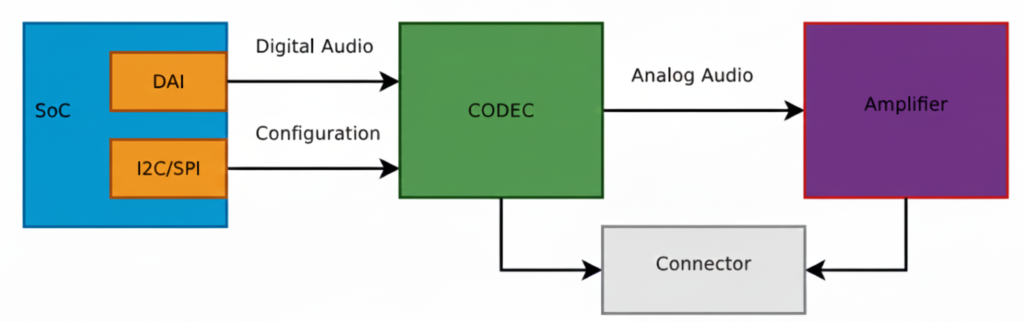
This diagram shows a typical embedded Linux / SoC audio playback architecture exactly the kind of pipeline you deal with in ALSA, QNX audio, codec drivers, and board bring-up. Let’s break it block by block, signal by signal, and then connect it to real software components you use.
SoC (System on Chip)
The SoC is the brain of the system (Qualcomm, TI, NXP, STM32MP, etc.).
Inside the SoC, two important blocks are shown:
DAI (Digital Audio Interface)
This block is responsible for sending and receiving digital audio samples.
Typical interfaces:
I2S
TDM
PCM
DSP_A / DSP_B
What flows here?
Raw PCM samples
Example: 16-bit / 24-bit / 32-bit audio
Sample rates: 44.1 kHz, 48 kHz, 96 kHz
Signals on the wire:
BCLK (Bit clock)
LRCLK / FS (Frame sync)
DATA
This is high-speed, real-time audio data
I2C / SPI (Control Interface)
This is NOT audio data.
Used only for:
Configuring the codec
Setting volume
Power control
Selecting input/output paths
Muting, unmuting
Clocking modes
Example operations:
Set DAC sample rate
Enable headphone output
Set gain = +6 dB
Power up analog blocks
This is low-speed control, not streaming audio.
Digital Audio Path (SoC → CODEC)
The arrow labeled “Digital Audio” represents:
SoC DAI ──(I2S/TDM/PCM)──> CODEC
✔ Audio is still digital ✔ No voltage amplification ✔ No sound yet
This is where:
ALSA PCM writes happen
DMA transfers audio buffers
Timing is critical
In ALSA terms:
CPU DAI ↔ Codec DAI
Defined in ASoC machine driver
Linked using snd_soc_dai_link
CODEC (Most Important Block)
The CODEC (Coder–Decoder) is the heart of audio hardware.
What the CODEC does:
DAC: Digital → Analog (playback)
ADC: Analog → Digital (capture)
Filtering
Mixing
Volume control
Clock management
Inputs:
Digital audio (I2S/TDM)
Control commands (I2C/SPI)
Outputs:
Analog audio signals (line-level)
Important:
The codec output is NOT strong enough to drive speakers
That’s why the next block exists.
Analog Audio Path (CODEC → Amplifier)
The arrow labeled “Analog Audio” means:
Audio is now continuous voltage
Typical level: ~1 Vrms (line level)
Sensitive to noise, grounding, layout
Signals here:
Left / Right analog outputs
Differential or single-ended
Amplifier
The Amplifier increases signal power so it can:
Drive speakers
Drive headphones
Overcome impedance
Amplifier types:
Class D (most common in embedded)
Class AB
Headphone amps
What it does:
Voltage amplification
Current amplification
Power delivery
Example:
Codec output: 1V
Amplifier output: 5–12V swing (speaker)
Connector (Speaker / Headphone Jack)
The Connector is the physical output:
Speaker connector
3.5mm headphone jack
Line-out
Automotive speaker terminals
Why shown separately? Because:
Board routing matters
ESD protection is added
Jack detection may exist
Multiple outputs can be routed
Full Signal Flow (End-to-End)
Playback path:
Application (aplay / media app)
        ↓
ALSA PCM
        ↓
CPU DAI (SoC)
        ↓  [Digital Audio: I2S/TDM]
CODEC (DAC)
        ↓  [Analog Audio]
Amplifier
        ↓
Speaker / Headphones
Software Mapping (Very Important)
In Linux ALSA ASoC:
Hardware Block
Software Component
SoC DAI
CPU DAI driver
CODEC
Codec driver
I2C/SPI
Regmap
Connections
Machine driver
User app
aplay, arecord
Why WAV is Used for Testing
WAV = raw PCM
No decoding needed
Direct match to DAI data
Perfect for testing this pipeline
MP3/AAC would require:
Decoder
Extra CPU
More variables
Big Picture Audio Hardware Block Diagram
Microphone
   ↓
[ Analog Front End ]
   ↓
ADC  →  SoC / MCU  →  DAC
   ↑        ↓        ↓
 Codec   DSP / CPU  Amplifier
                         ↓
                      Speaker
Let’s explain each block in detail.
Audio Input Hardware (Sound Capture)
Microphone
Converts sound waves → electrical signals
Types:
Electret Condenser Mic (analog output)
MEMS Mic
Analog MEMS
Digital MEMS (PDM / I2S output)
Key parameters:
Sensitivity (dBV/Pa)
Signal-to-noise ratio (SNR)
Directionality (Omni / Uni-directional)
Analog Front End (AFE)
Before audio reaches the ADC, it must be conditioned.
AFE includes:
Pre-amplifier (boosts weak mic signals)
Biasing circuit (for electret mics)
Low-pass filter (anti-aliasing)
Noise filtering
Without AFE, captured audio will be noisy or distorted.
Audio Codec (Heart of Audio Hardware)
What is an Audio Codec?
A codec = Coder + Decoder
It usually integrates:
ADC (Analog → Digital)
DAC (Digital → Analog)
Mixers, volume control, mute
Power management
Examples:
TLV320 series (TI)
PCM5102, PCM1808
WM8960
Realtek codecs
Why Codec Is Important
MCU/SoC cannot directly handle analog audio
Codec ensures:
Correct sampling
Bit depth
Clean audio conversion
Digital Audio Interfaces (SoC ↔ Codec)
Audio data moves digitally between SoC and codec.
I2S (Most Common)
Used for PCM audio.
Signals:
BCLK (Bit Clock)
LRCLK / WS (Left-Right clock)
DATA
MCLK (optional)
SoC  ←→  Codec
 I2S     I2S
Other Audio Interfaces
PCM/TDM – multi-channel audio (automotive, pro audio)
PDM – digital microphone interface
SPDIF – consumer audio
AC97 / HDA – PC-class audio
Audio Processing Hardware
MCU / SoC
Processes audio samples.
Responsibilities:
Buffer management
DMA handling
Audio routing
Running DSP algorithms
Examples:
BeagleBone (AM335x)
STM32F4/F7/H7
ESP32
Qualcomm SoCs
DSP (Optional but Powerful)
Dedicated processor for:
Noise cancellation
Echo cancellation
Equalizer
Compression
In many SoCs, DSP is integrated.
Audio Output Hardware (Sound Playback)
DAC
Converts digital PCM samples → analog waveform
Parameters:
Resolution (16-bit / 24-bit)
Sampling rate
Dynamic range
Often integrated inside codec.
Audio Power Amplifier
Boosts low-level analog signal to drive speakers.
Examples:
LM386 (you’ve used this)
TPA3116
Class-D amplifiers
Why needed?
Codec output ≈ millivolts
Speaker needs watts
Speaker / Headphones
Final sound-producing component.
Considerations:
Impedance (4Ω, 8Ω)
Power rating
Mono vs stereo
Clocking Hardware (Very Important)
Audio hardware needs precise clocks.
Sources:
External crystal
SoC PLL
Codec internal PLL
Clock affects:
Sampling accuracy
Audio quality
Jitter
Power Management in Audio Hardware
Audio is sensitive to power noise.
Hardware includes:
Separate analog & digital power rails
LDOs
Ground separation (AGND / DGND)
Bad power = hiss, pop, distortion.
Real Embedded Example (BeagleBone + Codec)
Mic → AFE → Codec ADC
               ↓
           I2S Bus
               ↓
        AM335x (ALSA)
               ↓
           I2S Bus
               ↓
           Codec DAC
               ↓
          LM386 Amp
               ↓
            Speaker
Software controls:
ALSA drivers
Device Tree
Mixer settings
Common Embedded Audio Hardware Issues
No sound → clock misconfiguration
Distorted audio → wrong gain
Noise → poor grounding
Channel swap → LRCLK mismatch
Crackling → buffer underrun
Summary
Block
Purpose
Microphone
Capture sound
AFE
Condition analog signal
ADC
Convert to digital
Codec
Audio conversion + control
I2S/PCM
Transfer digital audio
SoC/DSP
Process audio
DAC
Convert to analog
Amplifier
Boost signal
Speaker
Play sound
What is an Audio CODEC?
Codec = ADC + DAC + mixers + clocks + controls
CODEC = COder + DECoder
An audio codec is a single chip that can:
Record sound → convert analog sound into digital data
Play sound → convert digital data back into analog sound
It acts as a bridge between the real (analog) world and the digital world.
Controlled via:
I2C / SPI → registers
I2S / TDM → audio data
Why do we need a CODEC?
Microcontrollers / SoCs cannot understand analog voltages directly.
Microphone → gives analog voltage
Processor → understands digital numbers
Speaker → needs analog voltage
So we need a translator → that’s the CODEC.
Inside a CODEC: ADC + DAC
A codec internally contains:
ADC (Analog to Digital Converter)
Takes analog voltage (from mic/line-in)
Converts it into digital samples
Used during audio capture / recording
DAC (Digital to Analog Converter)
Takes digital samples
Converts them into analog voltage
Used during audio playback
Both ADC and DAC are inside one chip → called an Audio CODEC
What exactly does a CODEC do?
Recording path
Microphone → Analog voltage → ADC → Digital samples → SoC
Playback path
SoC → Digital samples → DAC → Analog voltage → Speaker / Amplifier
How does a CODEC talk to the SoC? (DAI)
CODECs don’t send data randomly. They use a Digital Audio Interface (DAI).
DAI is a synchronous serial interface (everything happens on clock edges).
Common DAI standards:
I²S
PCM
TDM
PCM / I²S Interface Basics
The 2 Main Clocks
Bit Clock (BCLK / BCK)
Ticks once per bit
Controls bit-by-bit transfer
Frame Clock (LRCLK / FSCLK / WCLK)
Ticks once per audio sample
Indicates Left / Right channel
Its frequency = Sample Rate (Fs)
Example:
Fs = 48 kHz → 48,000 samples per second
Relationship Between Clocks
Formula:
BCLK = FS × Number_of_Channels × Bit_Depth
Example:
Sample Rate (Fs) = 48 kHz
Channels = 2 (Stereo)
Bit depth = 16 bits
BCLK = 48,000 × 2 × 16 = 1.536 MHz
BCLK must run much faster than LRCLK.
Data Lines (Audio Data)
Along with clocks, we have data lines:
Carry the actual audio bits
Usually called: SDATA, DSDATA, ASDATA
Important points:
One data line can carry two channels (Left + Right)
Some codecs have multiple data lines:
One per channel pair
Useful for multi-channel audio
Multiple DAI Interfaces
Some codecs support:
Separate DAI for input (ADC)
Separate DAI for output (DAC)
This allows:
Different clocks
Different sample rates
Independent routing
Real Example: AD1937 CODEC
Capabilities
8 DAC channels → 4 stereo output pairs
4 ADC channels → 2 stereo input pairs
Playback (DAC side)
Clocks:
ABCLK → Bit clock
ALRCLK → Frame clock
Data lines:
ASDATA[1–2] → 2 output data lines
Capture (ADC side)
Clocks:
DBCLK
DLRCLK
Data lines:
DSDATA[1–4] → 4 input data lines
Perfect for multi-channel professional audio systems
Control Interface (Configuration Bus)
Audio data ≠ configuration.
CODECs use a separate control bus to:
Set volume
Select sample rate
Enable ADC/DAC
Configure routing
Common control buses:
I²C
SPI
Audio flows on DAI, configuration happens on I²C/SPI.
Left-Justified is a digital audio data format used to transfer audio samples between a codec and a SoC/DSP over serial audio interfaces like:
I²S
TDM
PCM interfaces
It defines how audio bits are aligned with the clock signals.
The 3 Important Audio Signals (Recap)
In any digital audio interface, you’ll see:
Signal
Meaning
BCLK
Bit Clock – clocks each bit
LRCLK / WS
Left-Right Clock (Word Select)
DATA
Actual audio sample bits
Left-Justified format describes when DATA starts relative to LRCLK.
Left-Justified Format – Core Idea
The MSB (Most Significant Bit) of the audio sample appears immediately after the LRCLK transition.
Key Rule:
No delay
MSB is aligned with the LRCLK edge
Data is “left-aligned” in the word frame
Timing Diagram (Conceptual)
LRCLK:  |____ LEFT ____|____ RIGHT ____|
            ↑                ↑
           MSB              MSB
BCLK :  |‾|_|‾|_|‾|_|‾|_|‾|_|‾|_|
DATA :  [MSB ........ LSB][MSB .... LSB]
As soon as LRCLK changes:
Data starts immediately
First bit = MSB
Example: 16-bit Audio Sample
Assume:
Sample size = 16 bits
Left channel sample = 0x5A3C
Bit Transmission (Left Channel)
LRCLK = 0  → LEFT channel
DATA   = 0 1 0 1 1 0 1 0 0 0 1 1 1 1 0 0
          ↑
         MSB (no delay!)
Left-Justified vs I²S (Very Important Interview Point)
Feature
Left-Justified
I²S
MSB position
Immediately after LRCLK edge
1 BCLK delay
Alignment
Left aligned
Delayed
Simplicity
Simple
Slightly complex
Codec support
Older & simple codecs
Most modern codecs
This 1-bit delay is the ONLY difference — but it breaks audio if misconfigured.
Why is it Called “Left-Justified”?
Because:
Audio data is pushed to the left side of the word frame
No padding before MSB
Extra unused bits (if any) come after LSB
Example (24-bit sample on 32-bit frame):
[ MSB .... LSB ][ 0 0 0 0 0 0 0 0 ]
Where is Left-Justified Used?
Common in:
Audio codecs (TLV320, PCM series)
Simple DAC/ADC interfaces
Embedded SoCs during codec bring-up
Some QNX / ALSA hardware configs
You’ll often see it as:
LEFT_J
LEFT_JUSTIFIED
LJ
ALSA / Embedded Perspective (Real World)
In ALSA, Left-Justified is configured using:
DAI format flags
Example:
SND_SOC_DAIFMT_LEFT_J
If:
Codec = Left-Justified
SoC = I²S
Audio will be distorted or silent
Simple One-Line Definition (Interview Ready)
Left-Justified audio format is a digital audio data format where the MSB of the sample appears immediately after the LRCLK transition, with no bit delay.
What is Right-Justified (RJ) Audio Digital Format?
Right-Justified is a digital audio data alignment format used to transfer audio samples between:
Codec ↔ SoC / DSP
Over interfaces like I²S, PCM, TDM
It defines how audio bits are aligned with the LRCLK (Word Select) signal.
Core Idea (Very Important)
In Right-Justified format, the LSB (Least Significant Bit) of the audio sample is aligned with the end of the LRCLK period.
Meaning:
Data is right-aligned
MSB position depends on sample width
Signals Involved
Signal
Role
BCLK
Clocks each bit
LRCLK / WS
Selects Left or Right channel
DATA
Audio sample bits
Right-Justified format defines where the LSB appears relative to LRCLK.
Timing Concept (Simple View)
LRCLK:  |____ LEFT ____|____ RIGHT ____|
                     ↑                ↑
                    LSB              LSB

BCLK :  |‾|_|‾|_|‾|_|‾|_|‾|_|‾|_|
DATA :  [MSB .... LSB][MSB .... LSB]
Padding bits come before MSB Sample ends exactly at LRCLK edge
Why “Right-Justified”?
Because:
Audio data is aligned to the right side of the frame
Extra unused bits are placed before MSB
LSB touches the LRCLK boundary
Right-Justified vs Left-Justified vs I²S
Feature
Left-Justified
Right-Justified
I²S
MSB alignment
Immediately after LRCLK
Variable
1 BCLK delay
LSB alignment
Variable
At LRCLK edge
Fixed
Padding bits
After LSB
Before MSB
After LSB
Common usage
Some codecs
Legacy codecs
Most modern systems
Important Embedded Detail
In Right-Justified, the SoC must know sample width:
16-bit
20-bit
24-bit
If sample width mismatches:
Audio distortion
Shifted samples
Noise / silence
This is why RJ is more error-prone than LJ or I²S.
ALSA / Driver Perspective
In ALSA SoC drivers, Right-Justified is selected using:
SND_SOC_DAIFMT_RIGHT_J
Typical usage:
Old DACs / ADCs
Simple PCM audio paths
Some automotive codecs
One-Line Interview Definition
Right-Justified audio format aligns the LSB of each audio sample with the LRCLK edge, while MSB position depends on the sample width.
Quick Memory Trick
Left-Justified → MSB touches LRCLK
Right-Justified → LSB touches LRCLK
I²S → MSB delayed by 1 BCLK
What is I2S (Inter-IC Sound)?
I2S (Inter-IC Sound) is a digital audio communication protocol used to transfer audio data between chips such as a processor, audio codec, DAC, or ADC.
Key Points of I2S
Designed specifically for digital audio
Transfers PCM (Pulse Code Modulation) audio data
Commonly used in embedded systems, SoCs, and audio boards
Simple and easy to implement
I2S Signals
I2S uses three or four lines:
BCLK (Bit Clock): Clocks each audio bit
LRCLK / WS (Word Select): Selects Left or Right audio channel
SD (Serial Data): Carries audio sample data
MCLK (Optional): Master clock for codec timing
I2S Features
Supports stereo audio (Left & Right)
Fixed channel structure
Low latency
Ideal for headphones, speakers, microphones
Where I2S is Used
Audio codecs (PCM, WM, TLV series)
Embedded Linux audio (ALSA)
Microcontrollers and DSPs
Music players and voice applications
What is TDM (Time Division Multiplexing)?
TDM (Time Division Multiplexing) is a digital audio interface that allows multiple audio channels to be transmitted over a single data line by assigning each channel a time slot.
Key Points of TDM
Supports multi-channel audio
Uses time slots instead of separate data lines
Highly scalable and efficient
Common in professional and automotive audio systems
TDM Signals
TDM typically uses:
BCLK (Bit Clock): Drives bit transmission
FS / SYNC (Frame Sync): Marks start of a frame
SD (Serial Data): Carries data for all channels
TDM Features
Supports 4, 8, 16, or more channels
Better bandwidth utilization
Reduces pin count on SoCs
Ideal for surround sound and voice systems
Where TDM is Used
Automotive infotainment systems
Multi-microphone arrays
Professional audio mixers
Advanced SoC audio pipelines
I2S vs TDM – Quick Comparison
Feature
I2S
TDM
Channels
2 (Stereo)
Multiple (4–16+)
Data Lines
One per stream
Single shared
Complexity
Simple
Moderate
Use Case
Basic audio
Multi-channel audio
Scalability
Limited
High
Summary
I2S is best for simple stereo audio communication
TDM is ideal for multi-channel, high-performance audio systems
Both are widely used in embedded audio, Linux ALSA, and SoC designs
Late data = noise Missing data = crack/pop Clock mismatch = drift
Key challenges:
Buffer underrun / overrun
Clock synchronization
Interrupt latency
DMA tuning
Playback vs Capture (Two Directions)
Playback
File → PCM → DAC → Speaker
Capture
Mic → ADC → PCM → File / Stream
Drivers must support both directions.
Compression vs Raw Audio
Type
Example
Used Where
Raw
PCM
Drivers, ALSA
Compressed
MP3, AAC
Apps
Lossless
WAV, FLAC
Storage
Embedded drivers almost never touch MP3/AAC.
Audio = Data + Time (Golden Rule)
Audio correctness depends more on TIMING than data
Even perfect samples are useless if late.
What is Clock in Audio?
In digital audio, a clock is a timing signal that synchronizes the transfer of audio data between components like a CPU, DSP, or audio codec. Without clocks, audio data could be misaligned, causing glitches, noise, or distortion.
Types of Clocks in Audio DAI (Digital Audio Interface)
Bit Clock (BCLK)
Drives the rate at which each audio bit is sent.
Think of it like the tick of a metronome, sending bits one by one.
Bit Clock Producer: One DAI (Digital Audio Interface) must generate this clock, called the BCLK producer (previously called “master”).
Frame Clock (LRCLK / Word Select / FS)
Signals the start of each audio frame (Left and Right channels in stereo).
Ensures the receiving device knows which bits belong to the left or right channel.
Frame Clock Producer: One DAI generates this, called the frame producer.
Master Clock (MCLK)
Optional but important for many CODECs.
Provides a high-frequency reference clock that other clocks (BCLK, LRCLK) can derive from using PLLs and dividers.
Helps CODECs generate precise bit and frame clocks even if the SoC provides multiple MCLK rates.
Who Should Generate the Clock?
Often, it’s better to let the CODEC act as the clock producer because:
CODECs have built-in PLLs and dividers for accurate BCLK from MCLK.
Reduces jitter (timing errors) in audio.
Some SoCs have specialized audio PLLs, so the CPU can generate precise clocks too.
Rule of thumb:
Let the device with the best PLL stability produce the clock.
The other device is called the bit or frame consumer, which simply follows the clock.
What are Auxiliary Devices in Audio?
In audio systems, auxiliary devices are additional hardware components that are not the main audio codec or processor, but help in modifying, routing, or amplifying audio signals. They can exist on the analog path (after digital-to-analog conversion) or sometimes on the digital path.
These devices are essential for fine-tuning audio output, volume control, or channel selection.
Types of Auxiliary Devices
Amplifiers
Boost the audio signal strength before sending it to speakers or headphones.
Examples:
Headphone amplifiers in mobile phones
Line amplifiers in sound cards
They can be controlled digitally in modern systems to adjust gain or mute audio.
Potentiometers (Volume Controls)
Analog knobs or digital controls that adjust signal amplitude.
They act as volume knobs or mixing controls.
Can be exposed in the ALSA sound card interface so software can control them.
Multiplexers (MUXes)
Switch between multiple audio sources or paths.
Example: Choosing between line-in, mic, or Bluetooth input.
Controlled via software registers to route audio correctly.
Other Analog Path Devices
Filters, equalizers, or attenuators
Ensure signal quality, reduce noise, or adjust frequency response
Control of Auxiliary Devices
Many auxiliary devices are software-controllable.
In ALSA (Advanced Linux Sound Architecture):
They appear as controls of the sound card.
Software can adjust volume, enable/disable paths, or switch inputs.
Input Source: Selects which audio path the multiplexer connects
This software abstraction makes it easy to manage analog devices programmatically.
Key Points for Beginners
Auxiliary devices are not the main audio codec, but they enhance or route audio.
They can be analog or digital controlled.
Exposing them as sound card controls allows software to adjust audio dynamically.
Common examples: Amplifiers, volume controls, multiplexers.
I2S (Inter-IC Sound) Interview Questions
Q1. What is I2S? Answer: I2S (Inter-IC Sound) is a digital audio interface used to transfer PCM audio data between chips such as processors, codecs, DACs, and ADCs.
Q2. How many signals does I2S use? Answer: I2S typically uses 3 or 4 signals:
BCLK (Bit Clock) – Clocks each audio bit
LRCLK / WS (Word Select) – Indicates Left or Right channel
SD (Serial Data) – Carries audio samples
MCLK (Master Clock) – Optional, used for codec timing
Q3. What audio formats does I2S support? Answer: I2S supports PCM audio, commonly 16-bit, 24-bit, or 32-bit samples, stereo only.
Q4. Difference between Left-Justified and I2S format? Answer:
I2S format: Data starts one clock after LRCLK changes.
Left-Justified: Data starts exactly at the LRCLK edge.
Q5. Where is I2S used in embedded systems? Answer:
Q1. What is TDM in audio? Answer: TDM allows multiple audio channels to share a single data line by assigning each channel a time slot, used for professional multi-channel audio.
Q2. How many channels can TDM support? Answer: It depends on the implementation; common configurations support 4, 8, 16, or more channels.
Q3. Difference between I2S and TDM? Answer:
Feature
I2S
TDM
Channels
2 (Stereo)
Multiple (4–16+)
Data lines
One per stream
Single shared
Complexity
Simple
Moderate
Use case
Basic stereo audio
Multi-channel audio
Q4. What signals are used in TDM? Answer:
BCLK (Bit Clock) – Synchronizes bits
FS / SYNC (Frame Sync) – Marks frame start
SD (Serial Data) – Carries all channels sequentially
Q5. Where is TDM commonly used? Answer:
Automotive infotainment
Multi-microphone voice capture
Surround sound systems
DSP audio pipelines
Practical/Scenario Questions
How do you connect an I2S codec to STM32?
Use BCLK, WS, SD pins, enable I2S peripheral, configure sample rate & word length.
How do you configure ALSA for TDM multi-channel audio?
Define codec and CPU DAI in ASoC machine driver, set number of slots, slot width, frame sync, and register in ALSA.
Why choose TDM over I2S?
When you need more than 2 channels over limited pins, e.g., 8-channel microphone arrays.
Explain Left-Justified vs Right-Justified format in I2S/TDM.
Left-Justified: Data aligned with LRCLK edge
Right-Justified: Data ends at LRCLK edge
Explore Embedded Audio Basics : From microphones to codecs, understand how audio works in embedded systems: Read more
Analog signal means the values can change smoothly over time (like a smooth wave).
2. Digital samples
Computers and embedded systems cannot understand continuous signals directly.
So, we convert analog sound into digital numbers, which are called samples.
This process is done by an Analog-to-Digital Converter (ADC).
Later, to play sound, the numbers are converted back to analog using a Digital-to-Analog Converter (DAC).
Simple example:
Imagine taking photos of a moving object every second. Each photo is a “sample” of the motion.
More photos = smoother playback; fewer photos = choppy motion.
Same idea with audio: more samples per second = better sound quality.
3. Timing constraints
Audio has to be played or processed at the right speed.
If the system is too slow or samples are missed, sound may become choppy, delayed, or distorted.
Embedded systems often use timers or buffers to ensure accurate timing while playing or recording audio.
Example:
If you play a song on your phone and it stutters or lags, it’s a timing problem.
Putting it all together
So, the formula:
Audio = Analog signal ⇄ Digital samples + timing constraints
means:
Audio starts as a real-world analog sound.
It is converted to digital samples so the system can process it.
It must be handled with proper timing to play correctly.
When needed, the digital samples are converted back to analog so we can hear it.
Understanding the Difference Between Sound and Audio
Sound is something we experience every day, whether it’s birds chirping, music playing, or a person talking. But in the world of electronics and embedded systems, you often hear the term audio. Many people wonder: Are sound and audio the same thing? Let’s break it down step by step.
What is Sound?
Sound is the natural phenomenon that we hear. It is created when an object vibrates, causing the surrounding air, water, or solid material to vibrate as well. These vibrations travel as waves, known as sound waves, which our ears detect.
Some key points about sound:
Sound is a physical wave in a medium (air, water, or solids).
It has frequency, which determines the pitch (high or low sound).
It has amplitude, which determines the loudness (soft or loud sound).
Real-world sounds often consist of many combined waves, giving each sound its unique quality, called timbre.
Examples: Clapping hands, a ringing bell, a dog barking.
What is Audio?
Audio is how we capture, process, store, or reproduce sound electronically. In simple terms, audio is sound converted into an electrical or digital form.
Some key points about audio:
Audio allows sound to be recorded, processed, transmitted, and played on electronic devices.
It can be analog (continuous electrical signal) or digital (numbers representing the sound).
Devices like microphones, speakers, computers, and smartphones use audio to handle sound in a usable form.
Examples: Songs on Spotify, voice recorded on a phone, sound effects in video games.
Sound vs Audio : Key Differences
Feature
Sound
Audio
Nature
Natural vibration in a medium
Electronic or digital form of sound
How we use it
Heard directly by humans
Processed, stored, or played via devices
Medium
Air, water, solids
Electrical signals or digital files
Example
Clapping hands, dog barking
MP3 song, recorded voice, podcast
Easy way to remember:
Sound is the real-world vibration we hear.
Audio is sound in a form that electronics can understand and use.
What is Audio
Audio is a time-varying analog signal representing air pressure variations, converted into electrical signals, then into digital data for processing, storage, and playback.
Audio Signal in the Real World (Physical Layer)
Sound → Air → Pressure Wave
Sound is a mechanical vibration
Travels as pressure waves
Human hearing range: 20 Hz – 20 kHz
Key properties:
Property
Meaning
Frequency
Pitch (Hz)
Amplitude
Loudness
Phase
Timing alignment
Audio in Embedded Systems (High-Level Flow)
Microphone
   ↓
Analog Front End (AFE)
   ↓
ADC (inside codec)
   ↓
Digital Audio (PCM samples)
   ↓
CPU / DSP / OS
   ↓
DAC (inside codec)
   ↓
Amplifier
   ↓
Speaker
Key idea: Your software never “plays sound” — it moves samples on time.
Sound waves are continuous
Sound waves are like smooth, endless curves.
They represent how air pressure changes over time when something makes a sound.
Continuous means the wave has an infinite number of points – it never “jumps” suddenly.
Measuring points on the wave
At any single point on the wave, you can measure how strong the sound is (its amplitude).
This single measurement is called a sample.
Think of it as taking a snapshot of the wave at one exact moment.
32-bit sample → used for special purposes, like precise calculations in audio processing.
6. Why Bit Depth Matters
More bits = more precision = smoother and more accurate sound.
Fewer bits → sound may be distorted or “grainy”.
That’s why 8-bit audio is rare today, while 16-bit and 24-bit are common.
Quick Summary
Concept
Explanation
Example
Sample value
Number representing amplitude at a moment
-1.0 to 1.0
Sample size (bits)
How many different values each sample can have
16-bit = 65,536 levels
Quality
More bits = better sound quality
8-bit = low, 24-bit = high
Analog vs Digital Audio (Critical Concept)
Analog Audio
Continuous voltage
Noise-prone
Example: microphone output
Digital Audio
Discrete samples
Binary data
Example: PCM buffer in RAM
Conversion happens using:
ADC (Analog → Digital)
DAC (Digital → Analog)
These are almost always inside an audio codec IC.
What is PCM? (This is your bread & butter)
PCM (Pulse Code Modulation) is raw, uncompressed audio data.
PCM = Samples taken at fixed intervals
Example:
Sample rate: 48 kHz
Bit depth: 16-bit
Channels: 2 (stereo)
Each sample:
Left sample | Right sample
In memory:
L0 R0 L1 R1 L2 R2 ...
PCM (Pulse Code Modulation) is a method to digitally represent analog audio signals. In simpler terms, it’s a way to take a continuous sound wave (like someone talking or music) and turn it into numbers that a computer or microcontroller can store, process, or transmit.
How PCM Works
Sampling
The analog signal is continuous over time.
PCM measures (samples) the signal at regular intervals, called the sampling rate.
Example: A sampling rate of 44.1 kHz (CD quality) means the audio is measured 44,100 times per second.
Quantization
Each sampled value is assigned a discrete number.
The number of bits used per sample determines the bit depth.
Example: 16-bit audio can represent 65,536 (2¹⁶) different amplitude levels.
Encoding
These discrete numbers are stored as binary data.
This sequence of numbers is your PCM audio stream.
Characteristics of PCM Audio
Linear PCM (LPCM): Most common type; samples are proportional to the original waveform.
Sample Rate: Higher rate → more accurate reproduction. Standard rates: 44.1 kHz, 48 kHz, 96 kHz.
Bit Depth: Higher depth → more dynamic range. Standard: 16-bit, 24-bit, 32-bit float.
Lossless representation of audio (no compression artifacts).
Standard for audio CDs, professional audio recording, and many embedded audio applications.
Easy to manipulate digitally (filtering, effects, mixing, etc.).
Example in Embedded Systems
Suppose you have a BeagleBone or STM32 and you want to play a recorded sound:
You store the audio in PCM format in memory (like an array of integers).
You send these samples to a DAC (Digital-to-Analog Converter) at the correct sample rate.
The DAC reconstructs the analog signal → goes to a speaker.
Key Audio Parameters (You MUST know these)
1. Sample Rate
Definition: The sample rate (or sampling frequency) is how many times per second the analog audio signal is measured (sampled) to convert it into digital form.
Unit: Hertz (Hz) → samples per second.
Example:
44.1 kHz → 44,100 samples per second (standard for audio CDs)
48 kHz → common in professional video and recording
96 kHz → high-resolution audio
Effect:
Higher sample rate → more accurate reproduction of the original waveform.
Lower sample rate → may lose high-frequency details (can cause aliasing if below Nyquist limit).
Embedded Example: If your microcontroller outputs 44,100 PCM samples per second to a DAC, it will reproduce the audio faithfully up to ~22 kHz (Nyquist theorem).
2. Bit Depth
Definition: Bit depth determines how many discrete levels are used to represent each audio sample.
Higher bit depth → more dynamic range (difference between softest and loudest sound)
Lower bit depth → more quantization noise
Embedded Example: If your STM32 DAC uses 12-bit resolution, each PCM sample must be mapped to 0–4095 levels.
3. Channels
Definition: Channels refer to the number of separate audio tracks in the PCM data.
Types:
Mono: 1 channel (same audio for all speakers)
Stereo: 2 channels (Left and Right)
Surround: 5.1, 7.1 channels → for multi-speaker systems
Effect:
More channels → more complex and immersive sound
Each channel has its own sample stream
Embedded Example: For stereo PCM audio on a microcontroller:
Left channel samples: [L1, L2, L3 …]
Right channel samples: [R1, R2, R3 …]
DAC outputs both channels to separate speakers simultaneously.
Summary Table
Feature
Definition
Effect
Example
Sample Rate
How many times per second audio is sampled
Accuracy of waveform
44.1 kHz
Bit Depth
Number of levels per sample
Dynamic range, quantization noise
16-bit
Channels
Number of separate audio tracks
Mono, stereo, surround
Stereo (Left + Right)
Shannon-Nyquist Theorem (Sampling Theorem)
Definition: The Shannon-Nyquist theorem states:
To digitally represent an analog signal without losing information, it must be sampled at a rate at least twice the highest frequency present in the signal.
To turn a real sound into digital data without losing any information, you need to “take enough snapshots” of the sound every second. The rule is: take at least 2 snapshots for every cycle of the fastest sound you want to capture.
Step by Step
Sound is a wave
Sound moves in waves (like ocean waves).
Each wave has a frequency: how fast it goes up and down per second.
Example: A piano note might be 440 Hz → 440 waves per second.
Digital can’t see continuous waves
Computers store numbers, not continuous waves.
So we “sample” the wave: take snapshots of its height at regular intervals.
How often should we take snapshots?
Shannon-Nyquist says: take at least twice as many snapshots as the highest frequency you want to capture.
Example: If the fastest sound is 20,000 Hz (human hearing limit), take at least 40,000 samples per second.
Why 2×?
If you take fewer samples, the wave can look like a completely different wave when you try to play it back.
This mistake is called aliasing.
Taking at least 2× ensures the original wave can be accurately recreated.
Super Simple Example
Imagine a bouncing ball going up and down 5 times per second.
If you take 2 photos per second → you might miss the motion → the ball looks weird.
If you take 10 photos per second → you see the motion clearly.
That’s basically Shannon-Nyquist for sound waves.
Formula:
Where:
(f_s) = sampling rate (samples per second)
(f_{max}) = maximum frequency in the analog signal
Why it matters
If you sample too slowly, higher frequencies in the signal will be misrepresented.
This misrepresentation is called aliasing.
Example:
Human hearing range: 20 Hz – 20 kHz
That’s why CDs use 44.1 kHz.
To capture all audible frequencies:
Aliasing Explained
If the sampling rate is below 2 *fmax
High-frequency components “fold back” into lower frequencies
The reconstructed audio sounds distorted
Visual: Imagine trying to sample a fast-moving wave slowly → it appears as a slower wave.
Embedded Systems Example
Suppose you have a microcontroller with a DAC:
You want to play a sound with frequency content up to 8 kHz
Minimum sample rate according to Shannon-Nyquist: (f_s \ge 16\text{kHz})
Using 16 kHz will reconstruct the waveform correctly
Using 10 kHz → aliasing will occur, audio will be distorted
Sound Digitization
Definition: Sound digitization is the process of converting an analog sound wave (continuous) into a digital format (numbers) that a computer can store, process, or play back.
Step 1: Sampling the Sound
The analog sound wave is measured at regular intervals.
Each measurement is called a sample.
Example:
A sound is recorded at 44.1 kHz → 44,100 samples per second.
Each sample captures the amplitude (height) of the wave at that instant.
Step 2: Quantization
Each sample is rounded to the nearest value that can be represented digitally.
This depends on bit depth.
16-bit → 65,536 possible levels
8-bit → 256 levels
Effect: Higher bit depth → more precise representation of the wave.
Step 3: Storing as WAV
WAV (Waveform Audio File Format) is a digital audio file format used to store audio in uncompressed PCM (Pulse Code Modulation) format.
Developed by Microsoft and IBM.
Stores raw audio data plus some metadata (like sample rate, bit depth, and number of channels).
Very common for high-quality audio in Windows and embedded projects.
WAV file is a common container for PCM audio.
Stores raw PCM data, along with metadata like:
Sample rate (e.g., 44,100 Hz)
Bit depth (e.g., 16-bit)
Number of channels (mono/stereo)
Structure of a WAV file (simplified):
[Header]       → info about sample rate, bit depth, channels
[Data Chunk]   → sequence of PCM samples
Understanding WAV Files: Beginner’s Guide to Digital Audio
Digital audio has become an integral part of technology, from music streaming and video production to embedded systems and microcontroller projects. Among various audio formats, WAV (Waveform Audio File Format) stands out for its simplicity, high quality, and ease of use. This article explains WAV files in a beginner-friendly way, covering their structure, usage, and technical details.
What Is a WAV File?
A WAV file is a digital audio file format that stores sound in an uncompressed PCM (Pulse Code Modulation) format. Unlike compressed formats such as MP3 or AAC, WAV preserves every detail of the original audio. This makes it ideal for high-quality audio playback, recording, and professional applications.
WAV files can store:
Mono or stereo audio
Different bit depths (8-bit, 16-bit, 24-bit, 32-bit)
Send them to a DAC at the correct sample rate to play the sound.
Common Audio Sample Rates and Their Uses
Sample Rate
Frequency Captured
Use / Typical Application
8 kHz
Up to 4 kHz
Telephony (phone calls), VoIP
16 kHz
Up to 8 kHz
Wideband voice, some low-quality audio
22.05 kHz
Up to 11 kHz
Low-quality music, older audio formats
32 kHz
Up to 16 kHz
FM radio, some lower-quality recordings
44.1 kHz
Up to 22 kHz
CD audio (standard for music), general-purpose audio
48 kHz
Up to 24 kHz
Video production, DVDs, broadcast audio
88.2 kHz
Up to 44.1 kHz
High-resolution audio, some studio recordings
96 kHz
Up to 48 kHz
Professional audio, film production, high-quality recording
192 kHz
Up to 96 kHz
Audiophile / ultra-high-resolution recordings
Guidelines for Choosing Sample Rate
Voice / telephony:
Use 8 kHz or 16 kHz → only needs human speech range (~300–3400 Hz).
Music / general audio:
Use 44.1 kHz → covers full human hearing (~20 Hz – 20 kHz).
Video / film:
Use 48 kHz → industry standard for audio/video sync.
High-quality / studio recording:
Use 96 kHz or 192 kHz → captures more details for professional mixing/mastering.
Embedded Systems Perspective
Microcontrollers with DACs often use 8 kHz–48 kHz.
Higher sample rates → better quality, but more memory and higher CPU load.
Example:
Playing music on a small MCU → 44.1 kHz, 16-bit stereo PCM
Voice alerts or notifications → 8 kHz, 8-bit mono PCM
Quick rule of thumb:
8–16 kHz: voice only
44.1 kHz: music / general audio
48 kHz: video / multimedia
96 kHz+: high-res studio recordings
Why we often use WAV files for testing audio instead of MP3, MP4, or other formats.
WAV Is Uncompressed (PCM)
WAV stores audio in raw PCM format—the exact waveform is preserved.
MP3, AAC, or MP4 are compressed formats (lossy or container formats), which remove some audio information to save space.
For testing audio in embedded systems or audio applications, you want the original waveform without any distortion from compression.
Example: If you are testing a DAC or audio pipeline, WAV ensures the numbers you send to hardware match the original waveform perfectly.
Simple Structure
WAV files have a simple, predictable header and straightforward data chunk.
You can read the samples directly into memory and send them to a DAC.
MP4 or MP3 files need decoding first (using codecs), which complicates testing.
In embedded systems, simplicity is key—WAV lets you focus on the hardware or playback pipeline without worrying about decoding software.
No Loss of Quality
Compression can introduce artifacts (unwanted noise or distortion).
Using WAV ensures that all audio details are preserved, which is crucial when testing:
DAC linearity
Speaker output quality
Signal processing algorithms
Predictable Timing
WAV files have a fixed sample rate and bit depth, so the timing of samples is predictable.
MP3/MP4 often use variable bit rates, which can make playback timing less precise—not ideal for testing embedded audio systems.
Industry Standard for Testing
Audio engineers and embedded developers almost always use WAV for test tones, audio calibration, and hardware verification.
Common test signals include:
Sine waves (to check frequency response)
Square waves (for DAC linearity)
White/pink noise (for speaker testing)
FAQs: What is Audio
1. What is audio? Audio is the representation of sound, either as a physical wave in air or as a digital signal. It can be captured, processed, stored, and played back in devices like computers, smartphones, and embedded systems.
2. How is audio captured from a microphone? A microphone converts sound waves into an analog electrical signal. This analog signal can then be converted into digital audio using an ADC (Analog-to-Digital Converter) and stored in formats like WAV or PCM.
3. What is PCM audio? PCM (Pulse Code Modulation) is a method of converting analog sound into digital form by sampling the amplitude of the sound wave at regular intervals and storing it as numbers.
4. What is the difference between WAV and MP3? WAV is an uncompressed audio format, preserving the original sound quality, making it ideal for testing and professional applications. MP3 is a compressed format that reduces file size but loses some audio details.
5. What is sample rate in audio? Sample rate is the number of times per second the analog signal is measured during digitization. Common sample rates are 44.1 kHz (CD quality) and 48 kHz (video/audio production).
6. What is bit depth in audio? Bit depth defines how accurately each audio sample is represented. Higher bit depth (like 16-bit or 24-bit) allows for greater dynamic range and more precise sound reproduction.
7. Why is WAV used for audio testing? WAV files store raw PCM audio without compression, ensuring exact waveform reproduction. This makes them perfect for testing audio hardware or embedded systems, where accuracy is crucial.
8. Can all captured audio be saved as WAV? Yes. Audio captured from a microphone or ADC can be saved as a WAV file by adding a header to the raw PCM data. Other formats like MP3 or AAC require compression and encoding.
9. What are the common audio channels? Audio can have one channel (mono), two channels (stereo), or more for surround sound setups (5.1, 7.1). Channels determine how sound is distributed across speakers.
10. How is audio used in embedded systems? Embedded systems use digital audio for alerts, notifications, music playback, and voice recognition. PCM data from WAV files is typically sent to a DAC to produce sound through speakers.
Recommended Resource: Expand Your ESP32 Knowledge
If you’re enjoying this project and want to explore more powerful sensor integrations, make sure to check out my detailed guide on using the ESP32 with the DS18B20 temperature sensor. It’s a beginner-friendly, real-world tutorial that shows how to measure temperature with high accuracy and integrate the data into IoT dashboards, automation systems, or cloud servers. You can read the full step-by-step guide here: ESP with DS18b20
This resource pairs perfectly with your ESP32 with RFID setup—together, you can build advanced smart home systems, environmental monitoring tools, or complete multi-sensor IoT projects.
Learn how to use ESP32 with LCD 16×2 step by step. Covers I2C and without I2C wiring, Arduino and MicroPython code, examples, and debugging tips.
Introduction
If you are working with ESP32, sooner or later you will want to show some data. Sensor values, WiFi status, IP address, time, menu options, or just a simple Hello World. That is where a 16×2 LCD display becomes your best friend.
Many beginners get stuck at the same questions:
Which LCD should I buy for ESP32?
Should I use I2C or connect it directly?
Why does my LCD show only blocks?
How do I write clean ESP32 LCD 16×2 code?
Can I use MicroPython?
Does this work in Wokwi simulation?
This guide answers all of that and more.
In this article, we will deeply explore esp32 with lcd 16×2, from basic wiring to real-world projects. You will understand not just how to connect things, but why they work. Think of this as a friend explaining things calmly over coffee, not a textbook.
ESP32 Description (Real-World Explanation)
ESP32 is a powerful microcontroller made by Espressif. It is not just a microcontroller. It is more like a small computer with WiFi and Bluetooth built in.
What makes ESP32 special:
Dual-core processor
Built-in WiFi and Bluetooth
Plenty of GPIO pins
Supports Arduino, MicroPython, ESP-IDF
Very affordable
Huge community support
In real life, ESP32 is used in:
IoT devices
Smart home systems
Industrial monitoring
Wearables
Robotics
Data loggers
Displays and dashboards
When you connect a 16×2 lcd display with esp32, you are basically giving eyes to your project.
ESP32 Pins Description
ESP32 has many pins, but not all are equal. Some are input only, some are safe at boot, and some can cause boot issues if misused.
Here is a simplified and practical ESP32 pins description table.
Pin Number
GPIO Name
Type
Notes
0
GPIO0
IO
Boot mode pin
2
GPIO2
IO
Onboard LED on some boards
4
GPIO4
IO
Safe to use
5
GPIO5
IO
SPI CS
12
GPIO12
IO
Boot sensitive
13
GPIO13
IO
Safe
14
GPIO14
IO
SPI CLK
15
GPIO15
IO
Boot sensitive
16
GPIO16
IO
Safe
17
GPIO17
IO
Safe
18
GPIO18
IO
SPI
19
GPIO19
IO
SPI
21
GPIO21
IO
I2C SDA
22
GPIO22
IO
I2C SCL
23
GPIO23
IO
SPI
25
GPIO25
IO
DAC
26
GPIO26
IO
DAC
27
GPIO27
IO
Safe
32
GPIO32
IO
ADC
33
GPIO33
IO
ADC
34
GPIO34
Input only
ADC
35
GPIO35
Input only
ADC
For esp32 with lcd 16×2 i2c, GPIO21 and GPIO22 are most commonly used.
What is a 16×2 LCD and How It Works
A 16×2 LCD means:
16 characters per row
2 rows total
Most of these displays are based on the HD44780 controller.
You do not need to memorize HD44780 datasheets. Just understand this:
The LCD has memory for characters
Each character is a 5×8 pixel pattern
You send commands and data
The controller handles the rest
When you write:
lcd.print("ESP32");
You are telling the LCD controller to place character patterns on the screen.
This is why interfacing 16×2 lcd module with esp32 is still popular after decades. It is simple and reliable.
LCD for ESP32: I2C vs Without I2C
This is one of the most confusing parts for beginners.
Without I2C (Parallel Mode)
Uses 6 to 10 GPIO pins
More wiring
Faster in theory
Harder for beginners
With I2C Module
Uses only 2 GPIO pins
Very clean wiring
Easy for beginners
Slightly slower but irrelevant for LCD
Comparison Table
Feature
I2C LCD
Normal LCD
Pins used
2
6 to 10
Wiring
Simple
Complex
Libraries
Easy
Medium
Beginner friendly
Yes
No
Recommended
Yes
Only if needed
For most projects, esp32 16×2 lcd with i2c is the best choice.
LCD 16×2 Connection with ESP32
I2C LCD Connection
LCD I2C Pin
ESP32 Pin
VCC
5V or 3.3V
GND
GND
SDA
GPIO21
SCL
GPIO22
This setup is used in esp32 lcd display 16×2 projects everywhere.
Without I2C Connection
You will need these pins:
RS
EN
D4
D5
D6
D7
This is used in esp32 lcd 16×2 without i2c projects.
This esp32 led example is often combined with LCD status messages.
LCD vs OLED with ESP32
LCD
Cheap
Easy
Text only
Sunlight readable
OLED
High contrast
Graphics support
More expensive
Burn-in risk
Use esp32 oled code when you need graphics. Use LCD for simple data.
Real-World Use Cases and Project Ideas
Temperature and humidity display
WiFi status screen
Smart meter display
Industrial parameter monitor
IoT dashboard
Menu-based user interface
Data logger status
Projects with esp32 with 16×2 lcd are still extremely relevant.
FAQ
Can ESP32 power a 16×2 LCD?
Yes, especially I2C modules. Some need 5V for backlight.
Why does my LCD show black boxes?
Contrast is wrong or initialization failed.
Which library is best?
LiquidCrystal_I2C is simple and stable.
Can I use ESP32 with LCD and WiFi together?
Yes, very common use case.
Is I2C slower?
Yes, but irrelevant for text displays.
Final Practical Conclusion
Using esp32 with lcd 16×2 is one of the best ways to learn embedded systems properly. It teaches you GPIO, I2C, libraries, debugging, and real-world thinking.
If you are a beginner, start with I2C. If you are advanced, understand both methods. If you are professional, use LCDs where reliability matters.
Once you master this, displays will never feel scary again.
Recommended Resource: Expand Your ESP32 Knowledge
If you’re enjoying this project and want to explore more powerful sensor integrations, make sure to check out my detailed guide on using the ESP32 with the DS18B20 temperature sensor. It’s a beginner-friendly, real-world tutorial that shows how to measure temperature with high accuracy and integrate the data into IoT dashboards, automation systems, or cloud servers. You can read the full step-by-step guide here: ESP with DS18b20
This resource pairs perfectly with your ESP32 with RFID setup—together, you can build advanced smart home systems, environmental monitoring tools, or complete multi-sensor IoT projects.
Master real pointer interview questions in c for embedded and linux roles with clear examples, common traps, coding questions, and memory-level explanations.
Pointers are one of the most important and most challenging topics in C programming interviews, especially for Embedded Systems, Linux System Programming, Linux Device Drivers, and RTOS (QNX / FreeRTOS) roles. A strong understanding of pointers is often the deciding factor between clearing and failing technical interviews.
This in-depth article on Pointer Interview Questions in C is designed as a complete beginner-to-advanced interview preparation guide. It covers every pointer concept that interviewers actually ask in real-world embedded and Linux interviews, explained in a simple, structured, and interview-oriented manner.
The article starts with pointer basics, including what pointers are, why they are required in C, pointer size, NULL pointers, void pointers, wild pointers, and dangling pointers. From there, it gradually moves into memory-level understanding, explaining how pointers interact with stack and heap memory, how memory leaks occur, and how improper pointer handling can crash embedded systems and long-running Linux services.
You will then learn pointer arithmetic with clear examples, covering pointer increment, decrement, pointer subtraction, and common interview trick questions. The guide also explains the relationship between pointers and arrays, including 1D and 2D arrays, pointer to array vs array of pointers, and the most common traps asked in interviews.
Advanced sections focus on pointers and functions, function pointers, callbacks in embedded systems, pointers with structures, and linked list implementations used in real projects. A dedicated section explains pointers and strings, highlighting the difference between char * and char[], string literals, and common mistakes that cause segmentation faults.
For experienced engineers, the article dives deep into const and volatile pointers, double pointers, pointer typecasting, and strict aliasing rules, with real embedded use cases. It also covers pointers in embedded systems and Linux device drivers, including DMA buffers, memory-mapped I/O, volatile hardware registers, and safe pointer handling in kernel space.
To make the article interview-ready, it includes real coding questions with answers, pointer output questions, debugging scenarios, and common interview mistakes along with best practices to avoid them.
Whether you are a fresher, an embedded software engineer, or preparing for senior Linux/driver interviews, this article will help you master pointers confidently, avoid common pitfalls, and answer interview questions with clarity and confidence.
Pointer Interview Questions
Pointer Basic
What is a pointer?
Why do we need pointers in C?
What is the size of a pointer?
Does pointer size depend on data type?
Difference between:
int a;
int *p;
What is NULL pointer?
What is void * pointer?
Can a pointer point to another pointer?
How to declare and initialize pointers?
What happens if a pointer is not initialized?
Difference between NULL and 0
Why NULL is preferred over 0
Can we dereference a NULL pointer?
What is wild pointer?
What is dangling pointer?
Pointer & memory (Very important)
How pointers access memory internally?
What happens during pointer dereferencing?
Difference between stack and heap memory using pointers
Pointer pointing to:
stack variable
heap memory
static memory
What happens if stack memory goes out of scope?
Why dangling pointers are dangerous?
How to avoid dangling pointers?
What is memory leak related to pointers?
How to detect memory leak?
Why pointers are risky in embedded systems?
Pointer arithmetic (Interview favorite)
What is pointer arithmetic?
Why pointer increment depends on data type?
What happens when:
p++
p + 1
Difference between:
p++
++p
Can we add two pointers?
Can we subtract two pointers?
Why pointer arithmetic is allowed only within same array?
What happens if pointer goes out of bounds?
Explain pointer arithmetic with example
Pointers & arrays (Most asked)
Relationship between array and pointer
Difference between:
int arr[]
int *p
Why array name behaves like pointer?
Why array name is constant?
Can we increment array name?
Difference between:
arr
&arr
Pointer to array vs array of pointers
1D array with pointers
2D array with pointers
Pointer to 2D array declaration
Difference between:
int **p
int (*p)[N]
Why 2D arrays are tricky with pointers?
Pointers & functions (Critical)
Passing pointer to function – why?
Call by value vs call by reference
How pointers help modify actual arguments?
Passing array to function internally how it works?
Why size of array is lost in function?
How to return pointer from function?
Returning pointer to:
local variable (why wrong)
static variable (why safe)
heap memory (best practice)
Function pointer basics
Syntax of function pointer
Use cases of function pointers
Function pointers in callbacks
Pointers & structures (Embedded favorite)
Pointer to structure syntax
Difference between:
(*ptr).member
ptr->member
Why structure pointers are used?
Passing structure vs pointer to structure
Structure padding & alignment impact on pointers
Pointer to structure inside structure
Self-referential structure
Linked list implementation using structure pointers
Real-time use of structure pointers in drivers
Pointers & strings (Very common)
How strings are stored in C?
Difference between:
char str[]
char *str
Why string literal should not be modified?
Where string literal is stored?
Pointer vs array string behavior
strlen using pointer logic
strcpy using pointer
strcat using pointer
Difference between const char * and char *
Const & pointers (Confusion zone)
What is const pointer?
Difference between:
const int *p
int *const p
const int *const p
Why const is important in embedded?
How const protects memory?
Const correctness in APIs
Double Pointer
What is double pointer?
Why double pointer is needed?
Real use cases of double pointer
Double pointer in:
dynamic memory allocation
linked list modification
driver APIs
Difference between:
int *p
int **pp
Passing pointer by reference using double pointer
Pointers & DMA / hardware (Real embedded)
Why DMA buffers use pointers?
Pointer alignment issues in DMA
Volatile pointer usage in hardware registers
Pointer to memory-mapped registers
Why volatile is required with pointers?
Accessing peripheral registers using pointers
Pointer casting for register access
Risks of wrong pointer type in hardware
What is volatile pointer?
Difference between:
volatile int *p
int *volatile p
Why volatile is required for ISR?
Volatile with memory-mapped IO
What happens if volatile is not used?
Pointers & volatile (Trick questions)
Pointer typecasting rules
When pointer casting is required?
Casting void * to other pointer
Alignment issues with pointer casting
Risks of wrong pointer casting
Strict aliasing rule
Pointer aliasing problems
Pointers & typecasting (Advanced)
Why kernel uses pointers heavily?
copy_from_user and pointer safety
User space vs kernel space pointer
What happens if kernel dereferences user pointer?
How kernel validates pointer?
Pointer usage in file_operations
Buffer handling using pointers in drivers
Why NULL checks are mandatory in kernel
Pointer debugging (Real interview scenarios)
How to debug segmentation fault?
Common pointer bugs
How to detect:
null pointer dereference
dangling pointer
buffer overflow
Tools to debug pointer issues:
GDB
Valgrind
Pointer-related crash example explanation
Trick & output questions (Must practice)
Predict output of pointer code
Multiple pointer increment confusion
Pointer + array output problems
Pointer with sizeof operator
Pointer precedence issues
Undefined behavior examples
Real-world interview scenarios (Very important)
How pointers help reduce memory copy?
Why embedded systems rely heavily on pointers?
How pointer misuse can crash RTOS?
How pointer bug can hang kernel?
Best practices for pointer usage in production code
How you ensure pointer safety in your projects?
FAQ : Pointer Interview Questions
1. what is a pointer in c and why is it important for interviews?
A pointer is a variable that stores the memory address of another variable. Interviewers focus on pointers because they test understanding of memory, performance, and low-level behavior, which are critical in embedded and linux programming.
2. why do embedded and linux interviews focus so much on pointers?
Embedded and linux systems interact directly with memory and hardware. Pointers are used to access registers, manage buffers, handle drivers, and optimize performance, making them essential interview topics.
3. what is the difference between a pointer and an array in c?
An array allocates fixed contiguous memory, while a pointer stores an address and can be reassigned. Although array names behave like pointers in expressions, they are not the same in memory behavior.
4. what are null, wild, and dangling pointers?
A null pointer points to no valid memory, a wild pointer is uninitialized, and a dangling pointer points to memory that has already been freed. All three can cause crashes if not handled correctly.
5. why is pointer arithmetic allowed only within arrays?
Pointer arithmetic is defined only within the bounds of the same allocated memory block. Accessing memory outside an array leads to undefined behavior and is commonly checked in interviews.
6. what is a double pointer and where is it used?
A double pointer stores the address of another pointer. It is commonly used for dynamic memory allocation, modifying pointers inside functions, and managing data structures like linked lists.
7. why should we not return the address of a local variable?
Local variables are stored on the stack and get destroyed when the function returns. Returning their address results in a dangling pointer and undefined behavior.
8. what is the difference between const int *p and int *const p?
const int *p means the data cannot be modified, while int *const p means the pointer address cannot change. This distinction is frequently tested in interviews.
9. why is volatile used with pointers in embedded systems?
The volatile keyword prevents the compiler from optimizing memory accesses. It is required when pointers access hardware registers or shared memory updated by interrupts.
10. how do pointers work in linux device drivers?
Pointers are used to manage buffers, access kernel structures, and interact with hardware. Safe pointer handling is critical because invalid access can crash the entire system.
11. what are common pointer mistakes that cause segmentation faults?
Common mistakes include dereferencing null pointers, accessing freed memory, incorrect pointer arithmetic, and writing beyond allocated memory.
12. how can i prepare pointer questions effectively for interviews?
Focus on understanding memory behavior, practice pointer-based coding questions, analyze common bugs, and relate pointer concepts to real embedded or linux use cases.
Conclusion of Pointer Interview Questions
Pointers are one of the most decisive topics in c programming interviews, especially for embedded systems, linux system programming, and device driver roles. A strong grasp of pointers shows interviewers that you understand memory, performance, and low-level system behavior rather than just syntax.
By mastering pointer basics, memory handling, pointer arithmetic, arrays, functions, structures, const and volatile usage, and real-world embedded scenarios, you significantly reduce the chances of making critical mistakes during interviews. Many candidates fail not because pointers are complex, but because they rely on memorization instead of understanding how memory actually works.
If you can confidently explain pointer behavior, identify common bugs, and relate pointer usage to real embedded or linux examples, you stand out as a reliable and job-ready engineer. Focus on clarity, practice real coding questions, and always think in terms of memory and safety. With the right preparation, pointer questions become an opportunity to showcase your technical strength rather than a reason for rejection.
Recommended Resource: Expand Your ESP32 Knowledge
If you’re enjoying this project and want to explore more powerful sensor integrations, make sure to check out my detailed guide on using the ESP32 with the DS18B20 temperature sensor. It’s a beginner-friendly, real-world tutorial that shows how to measure temperature with high accuracy and integrate the data into IoT dashboards, automation systems, or cloud servers. You can read the full step-by-step guide here: ESP with DS18b20
This resource pairs perfectly with your ESP32 with RFID setup—together, you can build advanced smart home systems, environmental monitoring tools, or complete multi-sensor IoT projects.
Learn QNX Resource Managers step by step with real examples. Understand IPC, message passing, drivers, and how QNX services work in practice.
Introduction of QNX Resource Managers
If you are working with real-time systems, safety-critical software, or automotive platforms, you will eventually run into QNX. And when you do, one topic comes up again and again: Writing Device Drivers and Resource Managers in QNX.
This is where many engineers get confused.
Linux developers often expect kernel modules. Beginners expect something similar to microcontroller firmware. QNX does neither in the traditional way. Instead, QNX takes a very different approach that feels strange at first but makes a lot of sense once it clicks. If you are new to QNX, you will understand the basics without feeling overwhelmed. If you already have experience with embedded Linux or RTOS systems, you will understand why QNX does things differently and how to work with it confidently. We will cover device drivers, resource managers, QNX Neutrino IPC, and message passing step by step.
By the end, Writing Device Drivers and Resource Managers in QNX will feel logical instead of mysterious.
What Makes QNX Different from Linux Driver Models
The biggest mental shift when moving to QNX is accepting that the kernel is not the center of everything.
Microkernel philosophy
Linux uses a monolithic kernel. Most drivers live inside the kernel space. If a driver crashes, the system usually goes down with it.
QNX uses a microkernel. The kernel does very little:
Scheduling
Interrupt handling
Low-level IPC
Basic memory management
Everything else runs in user space.
Why drivers run in user space
In QNX, most device drivers and all resource managers are user-space processes. This gives you:
Fault isolation
Easier debugging
Ability to restart drivers without rebooting
Better system stability
If a QNX driver crashes, the kernel stays alive. You can restart the driver like a normal process.
Real-world advantages
This design is one of the main reasons QNX is used in:
Automotive infotainment
ADAS systems
Medical devices
Industrial controllers
Safety certification becomes more realistic when one faulty component cannot crash the whole system.
Understanding QNX Neutrino Architecture
Before you write a single line of code, you must understand how QNX Neutrino is structured.
Microkernel at the center
The QNX Neutrino microkernel is tiny and deterministic. It does not know about filesystems, drivers, or networking. Those are all separate processes.
Processes vs threads
Process: Has its own address space
Thread: Runs inside a process and shares memory
Most QNX drivers are single processes with one or more threads.
IPC fundamentals
Everything in QNX talks through IPC. This is not optional. It is the backbone of the system.
This is where QNX Neutrino IPC becomes critical. Instead of shared memory hacks or kernel callbacks, QNX relies on message passing.
Once you understand IPC, device drivers and resource managers start to feel natural.
What Is a QNX Device Driver
A QNX device driver is a program that controls hardware and exposes it to user applications.
Where drivers live
Unlike Linux kernel modules:
QNX drivers are user-space processes
They can be started and stopped like normal programs
They often live under /dev
QNX character driver explained
Most beginners start with a QNX character driver. These drivers:
Handle byte streams
Look like files
Support open, read, write, close
Examples:
UART drivers
I2C device access
Simple GPIO interfaces
Driver vs resource manager
This is important:
Device driver: Talks directly to hardware
Resource manager: Presents a file-like interface to applications
Often, a driver is implemented as a resource manager. This is why beginners get confused. In QNX, these concepts overlap by design.
Resource Managers Explained Like You’ve Never Heard Before
Think of a resource manager as a translator.
What they are
A resource manager:
Registers a pathname like /dev/mydevice
Waits for client requests
Handles read, write, ioctl, open, close
Responds using IPC
Why they exist
QNX treats everything as a resource. Files, devices, services. A resource manager lets your service behave like a file.
Applications do not care if they are talking to:
A real file
A hardware device
A software service
Feels like files, acts like services
This is the magic.
You can open() a device, but behind the scenes, a message is sent to your process. You handle it in your own code.
A simple QNX resource manager example could expose a temperature sensor as /dev/temp0. Applications just read it like a file.
QNX Message Passing and IPC Deep Dive
This section is the heart of QNX.
Why message passing matters
Everything depends on it:
Drivers
Resource managers
Filesystems
Networking
Understanding QNX message passing is more important than memorizing APIs.
Core IPC calls
MsgSend()
MsgReceive()
MsgReply()
Flow:
Client sends a message
Server receives it
Server replies
Client unblocks
This is synchronous and deterministic.
Pulses
Pulses are lightweight messages:
No reply needed
Used for events and notifications
Very fast
Drivers use pulses for interrupts, timers, and signals.
Why this model works
No shared memory races
Clear ownership
Predictable timing
Easier debugging
Once you embrace this, QNX starts to feel clean and intentional.
Step-by-Step: Writing a Simple QNX Character Driver
This is a QNX device driver tutorial at a conceptual level. Enough to understand the flow without drowning in boilerplate.
High-level flow
Initialize hardware
Create a dispatch structure
Attach a resource manager
Enter dispatch loop
Handle read and write requests
Key structures
dispatch_t
resmgr_attr_t
resmgr_connect_funcs_t
resmgr_io_funcs_t
These structures tell QNX how to route messages to your code.
Data flow explained simply
User app calls read()
Kernel converts it to a message
Message arrives at your driver
Your io_read() function runs
You copy data to client buffer
Reply is sent automatically
No kernel hacking. No syscall tables.
Step-by-Step: Writing a Simple Resource Manager
A resource manager is often easier than a full driver.
Dispatch loop
The dispatch loop waits for messages and routes them:
dispatch_block()
dispatch_handler()
resmgr_attach
This registers your path:
/dev/myresource
Sets permissions
Connects handlers
io_read and io_write
These functions do the real work:
Validate request
Copy data
Update offsets
This model scales from simple demos to production systems.
User Application Interaction
From the application side, everything looks familiar.
File I/O model
Applications use:
open()
read()
write()
ioctl()
They do not need to know about IPC.
Message passing directly
Advanced apps can use:
MsgSend()
Pulses
Shared memory
This is useful for high-performance or control-heavy systems.
Real example
An automotive audio service may:
Use file I/O for control
Use message passing for real-time events
Use shared memory for audio buffers
QNX lets you mix models cleanly.
Debugging Tips for QNX Drivers and Resource Managers
Debugging is easier than Linux if you know how to think.
Common mistakes
Forgetting to reply to messages
Blocking inside handlers
Incorrect permissions
Bad offset handling
Debugging mindset
Think in terms of messages, not function calls.
Ask:
Who sent this message?
Why is the client blocked?
Did I reply correctly?
Useful tools
slog2
pidin
on -f
gdb
Logs and process inspection go a long way.
Performance, Safety, and Reliability Considerations
This is why QNX exists.
Automotive focus
QNX dominates automotive because:
Fault isolation is real
Determinism is predictable
Certification is practical
Fault containment
If your driver crashes:
Kernel survives
Other services survive
System can recover
Real-time behavior
Message passing is deterministic. No hidden kernel locks. This matters for safety systems.
Common Beginner Mistakes
Treating QNX like Linux
Ignoring IPC fundamentals
Blocking inside resource manager callbacks
Overusing shared memory
Forgetting permission settings
Not handling offsets correctly
Mixing driver logic with application logic
Real-World Use Cases
Automotive
Audio routing services
CAN and Ethernet gateways
Sensor abstraction layers
Medical
Patient monitoring devices
Imaging systems
Safety-certified controllers
Industrial
PLC communication
Fieldbus interfaces
Motion control systems
Frequently Asked Questions of QNX Resource Managers
What is the difference between a device driver and a resource manager in QNX?
A driver controls hardware. A resource manager exposes services using a file-like interface. Many drivers are implemented as resource managers.
Is kernel programming required in QNX?
No. Most drivers run in user space.
Why does QNX use message passing instead of shared memory?
Message passing is deterministic, safe, and easier to reason about in real-time systems.
Can Linux developers learn QNX easily?
Yes, but they must unlearn kernel-centric thinking.
What is QNX Neutrino IPC used for?
All communication between processes, including drivers and applications.
Are QNX character drivers similar to Linux character drivers?
Conceptually yes, but implementation is completely different.
Can I restart a crashed driver without rebooting?
Yes. This is a core advantage of QNX.
How are interrupts handled?
Interrupts are delivered as pulses or messages to user-space drivers.
Is QNX suitable for high-performance systems?
Yes. Many production automotive systems use it today.
How do applications talk to resource managers?
Using standard POSIX file I/O or direct message passing.
Is QNX harder than Linux?
Different, not harder. Once IPC clicks, it feels simpler.
Do I need to write resource managers for everything?
No. Only when you want a file-like interface.
Conclusion
Writing Device Drivers and Resource Managers in QNX is not about learning obscure APIs. It is about understanding a philosophy.
QNX is built around isolation, message passing, and clarity. Drivers are not special kernel magic. They are well-behaved user processes that communicate through clean IPC.
Once you understand QNX Neutrino IPC, message passing, and the role of resource managers, the system becomes predictable and powerful.
If you are serious about automotive, safety-critical, or real-time systems, mastering Writing Device Drivers and Resource Managers in QNX is one of the most valuable skills you can develop.
Practice small examples. Read the messages. Think in terms of services, not kernels. That is how real QNX systems are built.
Recommended Resource: Expand Your ESP32 Knowledge
If you’re enjoying this project and want to explore more powerful sensor integrations, make sure to check out my detailed guide on using the ESP32 with the DS18B20 temperature sensor. It’s a beginner-friendly, real-world tutorial that shows how to measure temperature with high accuracy and integrate the data into IoT dashboards, automation systems, or cloud servers. You can read the full step-by-step guide here: ESP with DS18b20
This resource pairs perfectly with your ESP32 with RFID setup—together, you can build advanced smart home systems, environmental monitoring tools, or complete multi-sensor IoT projects.
FreeRTOS Bugs often cause devices to crash after days of uptime due to task, queue, interrupt, and memory issues. Learn real causes and proven fixes.
FreeRTOS systems often run perfectly for hours or even days before suddenly crashing, hanging, or resetting without warning. These failures are rarely caused by obvious bugs. Instead, they come from subtle FreeRTOS issues that only appear after long runtime, real workloads, and unpredictable timing between tasks, interrupts, and memory.
In this deep-dive article, a senior embedded systems engineer with over 10 years of real-world FreeRTOS debugging experience breaks down the top 7 FreeRTOS bugs that crash devices after 2–3 days of runtime. This is not a beginner tutorial or academic theory. Every bug discussed here is based on real production failures seen in automotive, industrial, and IoT devices.
You will learn why common FreeRTOS bugs stay hidden during testing, how scheduling and heap behavior change over time, and why interrupt timing and task interaction are the real culprits behind long-runtime crashes. The article explains stack overflows that do not crash immediately, queue misuse involving QueueHandle_t, busy wait loops that slowly starve the scheduler, incorrect interrupt priorities, memory corruption caused by missing memory barriers, event group misuse, and CAN bus deadlocks under load.
Each bug includes a real-world scenario, why it passes initial testing, the exact failure mechanism, how it leads to a hard fault, hang, or watchdog reset, and how both beginners and experienced developers accidentally introduce it. You will also learn practical detection techniques using FreeRTOS backtrace analysis, coredumps, GDB, Segger Embedded Studio, tracing tools, and debugger workflows that actually work in production environments.
This article is written for real developers who debug real systems. If you are dealing with unexplained FreeRTOS crashes, long-term stability issues, or devices that fail only after days of uptime, this guide will help you recognize the patterns, confirm the root cause, and fix the problem correctly without guesswork.
Introduction
If you have worked with FreeRTOS long enough, you have seen this pattern.
The device boots fine. Runs all tests. Survives stress testing. Customer deploys it. Two or three days later, it locks up, resets, or goes silent.
But scheduling creates time-based behavior, not immediate behavior. A task might run fine for 10,000 iterations before it finally collides with another task at just the wrong moment.
Heap behavior changes over time
Even if you never call pvPortMalloc() after startup, fragmentation can still happen indirectly.
Heap corruption rarely crashes immediately. It poisons memory slowly until something important gets overwritten.
Interrupt timing is never stable
What worked at low traffic fails under real load.
CAN bursts. Button spam. GPIO storms. DDS or sensor interrupts firing faster than expected.
That is why debugging FreeRTOS issues always requires thinking in timelines, not just code paths.
Top 7 FreeRTOS Bugs That Crash Devices After 2–3 Days
🐞 Bug #1: Stack Overflow That Does Not Crash Immediately
Real-world scenario
A task handles protocol parsing. It has a local buffer, some structs, maybe a JSON decode. Everything works.
After two days, device resets with a freertos hardfault.
Why it passes initial testing
Stack usage is almost enough
Typical test messages are smaller
Worst-case path is rare
FreeRTOS does not magically know your worst execution path.
Failure mechanism
Stack grows slowly over time. Eventually it overwrites:
Task control block
Queue structures
Event group memory
Now the scheduler trips over corrupted data.
Result
Random reset
Silent hang
Hard fault inside the kernel
When you finally capture it, the freertos backtrace looks meaningless.
Beginner mistake
Assuming default stack sizes are fine.
Experienced mistake
Adding “just a bit more stack” without measuring.
How to detect it
Enable stack overflow checking
Use uxTaskGetStackHighWaterMark
Inspect task stacks in freertos gdb or freertos segger embedded studio
If you ever use freertos+trace, stack usage spikes become obvious.
How to fix it
Measure worst-case stack usage
Avoid large local arrays
Move buffers to static memory
This alone eliminates a shocking number of freertos bugs.
🐞 Bug #2: Queue Misuse with QueueHandle_t
Real-world scenario
You use queues everywhere. Sensor task pushes data. Processing task pulls it. Clean design.
Two days later, tasks stop responding.
Why it passes initial testing
Queues hide errors extremely well.
Sending to a deleted queue. Using a stale freertos queuehandle_t. Sending from ISR without the ISR-safe API.
All of these may work… until timing shifts.
Failure mechanism
Queue internal structures get corrupted. Eventually scheduler walks invalid memory. Boom.
Result
Deadlock
Kernel assert
Hard fault
Often shows up as corrupted lists during debugging FreeRTOS.
Beginner mistake
Not checking return values from xQueueSend.
Experienced mistake
Passing queue handles across modules with no ownership rules.
How to detect it
Enable asserts
Validate queue handles
Capture freertos coredump and inspect queue internals
How to fix it
One owner per queue
Clear lifecycle rules
Use ISR APIs correctly
Queues are powerful, but they are not magic.
🐞 Bug #3: Busy Wait Instead of Proper Blocking
Real-world scenario
A task waits for hardware.
So someone writes:
while(!flag) {}
Classic freertos busy wait.
Why it passes initial testing
CPU is fast. Load is low. It “works”.
Failure mechanism
Busy wait:
Starves lower priority tasks
Prevents idle task from running
Blocks memory cleanup
Delays timers
Over days, timing drift builds up.
Result
Watchdog resets
Tasks never unblock
System slowly degrades
Beginner mistake
Not understanding freertos blocking APIs.
Experienced mistake
Using busy wait to “optimize latency”.
How to detect it
CPU usage stuck near 100%
Idle task not running
Trace shows starvation
How to fix it
Use:
vTaskDelay
xQueueReceive
freertos wait for event
FreeRTOS is event-driven. Fight that and it fights back.
🐞 Bug #4: Incorrect Interrupt Priorities
Real-world scenario
GPIO interrupt fires on button press. CAN interrupt fires on bus traffic. Everything works.
After heavy load, system crashes.
Why it passes initial testing
Interrupt timing is light. No nesting issues.
Failure mechanism
Wrong priority interrupts calling FreeRTOS APIs.
This violates kernel rules and corrupts internal state.
Result
Scheduler corruption
Random asserts
freertos hardfault
Often blamed on hardware.
Beginner mistake
Ignoring priority rules in interrupts FreeRTOS.
Experienced mistake
Porting code from another RTOS without rechecking priorities.
How to detect it
Audit ISR priorities
Check which ISRs call RTOS APIs
Debug with freertos debugger
How to fix it
Follow max syscall interrupt priority rules
Separate pure hardware ISRs from RTOS-aware ISRs
This bug alone explains many “it crashes only under load” cases.
🐞 Bug #5: Missing Memory Barriers
Real-world scenario
Shared data between ISR and task. Flags look correct. Logic is sound.
Still fails.
Why it passes initial testing
Compiler optimizations are minimal. Timing is lucky.
Failure mechanism
Without a freertos memory barrier, compiler or CPU reorders memory access.
Task sees stale data. ISR thinks task handled it.
Result
Missed events
Deadlocks
Random behavior
Very hard to reproduce.
Beginner mistake
Not understanding memory ordering.
Experienced mistake
Assuming volatile is enough.
How to detect it
Review shared variables
Look for lock-free code
Inspect assembly in freertos gdb
How to fix it
Use FreeRTOS synchronization primitives
Insert memory barriers where required
Avoid lock-free sharing unless necessary
This is one of the sneakiest freertos bugs.
🐞 Bug #6: Event Group Misuse
Real-world scenario
Multiple tasks wait on events. Button interrupt sets a flag. Processing task waits.
Using freertos events everywhere feels elegant.
Why it passes initial testing
Low contention. Clear logic.
Failure mechanism
Event bits cleared too early
Tasks waiting incorrectly with freertos wait for event
Missed signals
Eventually tasks block forever.
Result
Silent hang
System appears alive but does nothing
Beginner mistake
Using events like queues.
Experienced mistake
Over-clever event bit combinations.
How to detect it
Log event transitions
Use trace tools
Inspect blocked task lists
How to fix it
Use events only for signaling
Use queues for data
Keep event logic simple
🐞 Bug #7: CAN Bus Deadlocks
Real-world scenario
CAN RX interrupt pushes frames. Processing task sends responses.
Works fine until bus traffic spikes.
Why it passes initial testing
Test traffic is clean. No overload.
Failure mechanism
RX ISR blocks indirectly
TX queue fills
Tasks wait on each other
Classic freertos can bus deadlock.
Result
Bus silence
Tasks blocked forever
Watchdog reset
Beginner mistake
Doing too much inside CAN ISR.
Experienced mistake
Ignoring backpressure handling.
How to detect it
Monitor queue depth
Log ISR execution time
Inspect blocked tasks
How to fix it
Minimal ISR work
Dedicated CAN worker task
Proper flow control
Final Thoughts
If you are chasing a crash that happens after days, it is not random.
It is almost always:
Stack
Queues
Interrupts
Blocking
Memory ordering
Events
Bus contention
Every single item in this freertos bug list has caused real devices to fail in the field.
If you take one thing from this article, let it be this:
FreeRTOS does exactly what you tell it to do. Even when that destroys your system slowly.
Debug patiently. Trace behavior over time. Trust evidence, not assumptions.
And next time someone suggests a freertos bug bounty, you will know exactly where to look first.
FAQ on FreeRTOS Bugs
1. Why do FreeRTOS devices crash after 2–3 days of runtime?
Most long-runtime crashes are caused by hidden FreeRTOS Bugs such as slow stack overflows, queue misuse, interrupt priority mistakes, or memory corruption that only appears after repeated task execution and timing drift.
2. What are the most common FreeRTOS Bugs in production systems?
The most common FreeRTOS Bugs include task stack overflows, incorrect QueueHandle_t usage, busy wait loops instead of proper blocking, wrong interrupt priorities, event group misuse, and CAN bus deadlocks under load.
3. How can a stack overflow crash a FreeRTOS system without an immediate fault?
In FreeRTOS, a stack overflow often overwrites nearby kernel data instead of crashing instantly. The system keeps running until the scheduler or queue logic touches corrupted memory, leading to a delayed hard fault or reset.
4. How do I detect FreeRTOS Bugs that only happen after long uptime?
Enable stack overflow checks, use runtime stats, capture coredumps, and analyze task states with a FreeRTOS debugger. Long-runtime bugs usually require observing behavior over time, not just single execution paths.
5. Why is busy wait dangerous in FreeRTOS?
Busy wait loops prevent the scheduler and idle task from running properly. Over time, this starves lower-priority tasks, delays timers, increases CPU load, and eventually causes system instability or watchdog resets.
6. What happens if interrupt priorities are wrong in FreeRTOS?
If interrupts call FreeRTOS APIs from invalid priority levels, the kernel’s internal data structures can become corrupted. This often leads to random crashes, asserts, or hard faults that are very difficult to reproduce.
7. Can QueueHandle_t misuse really crash a FreeRTOS system?
Yes. Using invalid or stale QueueHandle_t values, sending to deleted queues, or using non-ISR-safe APIs inside interrupts can corrupt queue memory and eventually crash the scheduler.
8. How do FreeRTOS event groups cause deadlocks?
Event groups can cause deadlocks when bits are cleared too early, multiple tasks wait on the same event incorrectly, or events are used to pass data instead of just signals. This leads to tasks blocking forever.
9. Why do CAN bus issues appear after days in FreeRTOS systems?
Under heavy traffic, CAN receive interrupts, transmit queues, and processing tasks can block each other. Without proper flow control, FreeRTOS CAN bus handling can deadlock and silently stop communication.
10. What tools are best for debugging FreeRTOS Bugs?
GDB, Segger Embedded Studio, FreeRTOS trace tools, and coredump analysis are the most effective. These tools help inspect task states, backtraces, stack usage, and scheduler behavior over long runtimes.
11. Are FreeRTOS memory barriers really necessary?
Yes. Missing memory barriers can cause the compiler or CPU to reorder memory access between tasks and interrupts. This leads to subtle, timing-dependent bugs that appear only under real workloads.
12. Why do FreeRTOS Bugs pass testing but fail in the field?
Lab tests rarely reproduce real timing, interrupt frequency, bus load, or long-term memory behavior. FreeRTOS Bugs often depend on rare timing windows that only occur in real deployments.
13. Can FreeRTOS coredumps help with long-runtime crashes?
Absolutely. A FreeRTOS coredump allows you to inspect task stacks, queue states, and scheduler data at the moment of failure, which is critical for diagnosing crashes that happen after days.
Recommended Resource: Expand Your ESP32 Knowledge
If you’re enjoying this project and want to explore more powerful sensor integrations, make sure to check out my detailed guide on using the ESP32 with the DS18B20 temperature sensor. It’s a beginner-friendly, real-world tutorial that shows how to measure temperature with high accuracy and integrate the data into IoT dashboards, automation systems, or cloud servers. You can read the full step-by-step guide here: ESP with DS18b20
This resource pairs perfectly with your ESP32 with RFID setup—together, you can build advanced smart home systems, environmental monitoring tools, or complete multi-sensor IoT projects.