Learn how PID control works Proportional, Integral, and Derivative explained simply with real examples, tuning methods, and code. Perfect for beginners.
If you’ve ever wondered how a car cruise control stays locked at exactly 100 km/h on a hilly road, or how a drone hovers perfectly still in a gusty breeze, or how your home thermostat keeps the temperature from swinging wildly the answer to all three is the same thing: a PID controller. And once you understand it, you’ll start seeing it everywhere.
This guide is about understanding PID control explained in plain language. Whether you’re a hobbyist building your first Arduino project, an engineering student preparing for interviews, or a professional who wants to finally nail the intuition behind something you’ve been using for years this is for you.
What Is PID Control? Start Here Before Anything Else
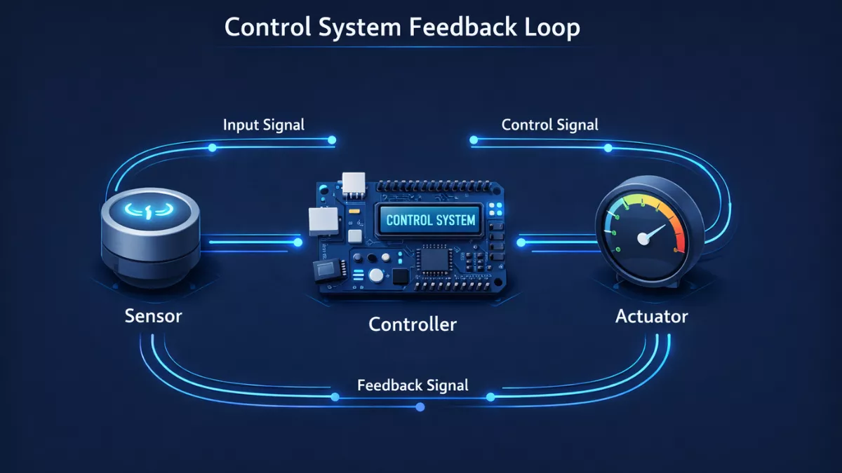
PID stands for Proportional, Integral, and Derivative. It’s a control loop mechanism a feedback-based algorithm that continuously calculates an error value as the difference between a desired setpoint and a measured process variable, then applies a correction based on three terms.
Imagine you’re driving a car and you want to maintain 80 km/h. Your eyes are checking the speedometer (that’s measurement), your brain compares what it sees to what you want (that’s error calculation), and your foot adjusts pressure on the accelerator (that’s the control output). You’re already doing PID in your head without knowing it.
The PID controller just does this automatically, much faster than a human can, and with mathematical precision. It reads a sensor, compares the reading to a target (called the setpoint), computes an error, and drives an actuator a motor, a heater, a valve, a servo to reduce that error as fast as possible without overshooting.
PID control is used in robotics, industrial automation, HVAC systems, drones, chemical plants, audio equipment, and even financial algorithms. One study estimated over 90% of industrial control loops use some form of PID control. That should tell you how fundamental this is.
The History Behind PID: Where It Came From and Why It Survived
PID control wasn’t invented overnight. The roots go back to the early 1900s. Elmer Sperry is often credited with early feedback control work on ship steering gyroscopes. But the formal mathematical framework for what we now call PID was developed by Nicolas Minorsky in 1922, who studied automatic ship steering for the U.S. Navy.
In the 1930s and 40s, Taylor Instrument Companies introduced pneumatic PID controllers for industrial process control. These were entirely mechanical air pressure changed based on error, and that pressure drove valves. Remarkably, the underlying logic was identical to what we implement digitally today.
By the 1980s, digital PID controllers became standard as microprocessors got cheap enough for industrial use. Today, every major PLC (Programmable Logic Controller) platform has PID blocks built in. Every embedded platform Arduino, STM32, Raspberry Pi has open-source PID libraries. The algorithm has been around for over a century and it’s still the go-to tool because it works, it’s simple to implement, and engineers understand how to tune it.
The Three Terms Explained: P, I, and D One at a Time
Proportional Control (P): React to What’s Happening Right Now
The proportional term is the simplest. It produces an output proportional to the current error. If the error is large, the output is large. If the error is small, the output is small.
Think of it like this: you’re trying to park a car in a tight spot. The farther away you are from the target position, the harder you press the reverse pedal. As you get closer, you ease off. That’s proportional action.
Mathematically: P output = Kp x error
Where Kp is the proportional gain. A higher Kp means a more aggressive response. The main limitation of pure proportional control is that it almost always leaves a steady-state error the system gets close but never quite reaches the setpoint. This is why we need the other two terms.
Integral Control (I): Remember the Past and Fix Accumulated Error
The integral term looks at the history of the error. It accumulates the error over time. If the error has been sitting at a small positive value for a long time, the integral term keeps building up, adding more corrective force until the system is actually driven to the setpoint.
Think of a room that’s slightly colder than you want. The heater is on but not quite powerful enough to hit the target. The integral term in the thermostat notices the room has been too cold for ten minutes, adds that up, and pushes the heater harder until it actually hits the target.
Mathematically: I output = Ki x (sum of all past errors x time)
The integral term eliminates steady-state error. But it comes with its own problem: integral windup. If the system has been in error for a long time, the integral can accumulate a huge value and cause the system to overshoot badly when it finally can respond. Anti-windup clamping is the standard fix.
Derivative Control (D): Predict the Future and Slow Down Before Overshooting
The derivative term reacts to the rate of change of the error, not the error itself. If the error is rapidly decreasing, the derivative term applies a braking force it slows the correction before the system reaches the setpoint, preventing overshoot.
Think of driving toward a stop sign. A smart driver starts braking before reaching the line. The derivative term is that braking — it detects that you’re approaching the target fast and applies reverse force to prevent overshoot.
Mathematically: D output = Kd x (rate of change of error)
The practical challenge with the derivative term is noise sensitivity. Almost all real sensors have some noise, and the derivative amplifies it, causing the actuator to chatter. That’s why many real-world implementations use a derivative filter or just run a PI controller instead.
The PID Equation: Putting All Three Terms Together
The full PID control equation is:
u(t) = Kp x e(t) + Ki x integral[e(t)dt] + Kd x de(t)/dt
- u(t) is the control output sent to the actuator
- e(t) is the error at time t (setpoint minus measured value)
- Kp, Ki, Kd are the gain parameters you tune
- The integral term accumulates past errors to eliminate steady-state offset
- The derivative term applies a braking force based on how fast the error is changing
In a digital system, this becomes a discrete-time approximation computed every fixed time step (the sample period). The quality of your PID implementation depends a lot on how consistently you run the loop. Use hardware timers or RTOS tasks with fixed periods — never delay() in your production PID code.
How a PID Controller Works in a Real System: Step by Step
Let’s trace through a complete PID control loop on a real example: controlling the speed of a DC motor using a microcontroller and an encoder.
- Measure: The encoder reads the current motor speed. Let’s say it measures 850 RPM.
- Calculate error: Setpoint is 1000 RPM. Error = 1000 – 850 = 150 RPM.
- Compute P term: With Kp = 0.5, P output = 0.5 x 150 = 75.
- Compute I term: Integral has accumulated. Say integrated value = 20, Ki = 0.1, so I output = 2.
- Compute D term: Error improved from 180 to 150 RPM this cycle. Rate = -3000 RPM/s. With Kd = 0.001, D = -3 (small brake).
- Sum: Total output = 75 + 2 + (-3) = 74. This maps to a PWM duty cycle that increases motor voltage.
- Wait for next sample period (10ms), read encoder again, repeat.
After several cycles, the motor converges on 1000 RPM and holds it there, even if load changes try to drag it down. That’s PID working in real time.
PID Tuning Methods: How to Actually Find the Right Gains
Manual Tuning: The Trial-and-Error Method
- Set Ki and Kd to zero. Start with only proportional control.
- Increase Kp until the system responds well and starts to oscillate. Back off Kp by about 50%.
- Add Ki slowly until steady-state error is eliminated. Watch for overshoot.
- Add Kd carefully if still seeing too much overshoot. Filter the derivative if the system chatters.
Ziegler-Nichols Method: The Classic Engineering Approach
Developed in 1942, this method gives you a systematic starting point:
- Set Ki and Kd to zero.
- Increase Kp until the system oscillates steadily. This is the Ultimate Gain (Ku).
- Note the oscillation period — the Ultimate Period (Tu).
- Apply Z-N formulas: Kp = 0.6 x Ku, Ki = 2 x Kp / Tu, Kd = Kp x Tu / 8.
This gives an aggressive controller with ~25% overshoot. You’ll still need to fine-tune, but you’ll be in the right ballpark. Caveat: pushing a system to the edge of instability isn’t always safe or acceptable.
Step Response / FOPDT Method: Model the System First
Apply a step input open-loop and record the output response. Extract three parameters: Process gain K (how much does output change per unit input), Dead time L (how long before output starts responding), Time constant T (time to reach 63% of final value). These describe a First Order Plus Dead Time (FOPDT) model. Published formulas like IMC-based tuning or Cohen-Coon convert K, L, T directly into PID gains without needing to push the system to oscillation.
Common PID Tuning Problems and How to Recognize Them
- Slow and sluggish response: Kp too low. Increase it. If still slow, Ki may also be too low.
- Oscillating around the setpoint: Kp too high. Back it off. If persists, Ki may also be too high.
- Large overshoot: Kp too high or Kd too low. Reduce Kp first. If still overshooting, add/increase Kd.
- Steady-state error: Ki is what you need. Increase it until error is eliminated, watching for overshoot.
- Chattering actuator: Derivative amplifying sensor noise. Add a low-pass filter to the sensor or the derivative calculation.
- Integral windup: After long error periods, system massively overshoots. Fix with anti-windup clamping.
Types of PID Controllers: Position vs Velocity Form
When you implement a PID controller in code, you have two main options:
Position Form PID: The standard form. The output at any time is the direct sum of P, I, and D terms, representing the absolute actuator position/value. Works fine for most applications. Challenge: if the controller restarts mid-operation, the output can jump suddenly because the integral was reset.
Velocity (Incremental) Form PID: Computes the change in output (delta) at each step rather than the absolute value. Naturally bumpless — if the controller switches on or the setpoint changes, there’s no sudden jump. Preferred in industrial applications for motor drives, valve positioners, or any system where sudden output changes cause mechanical stress.
PID Control in the Real World: Industry Applications
Temperature Control
Ovens, autoclaves, injection molding machines, chemical reactors, soldering stations, 3D printer hotends — all use temperature PID loops. Temperature systems are typically slow (high thermal mass), have significant dead time, and often don’t need the derivative term at all. A PI controller is usually sufficient and preferred to avoid amplifying thermocouple noise.
Motor Speed and Position Control
Servo drives, CNC machines, robotic joints — all use PID for speed control and often cascaded PID (inner speed loop, outer position loop) for precise positioning. Motor control loops run at high frequency (1 to 10 kHz is common), making discrete-time implementation details critical. Sample time jitter can cause noticeable degradation in control quality.
Drone Flight Control (Attitude Control)
Every commercial drone uses PID control to maintain attitude (roll, pitch, yaw) and altitude. The gyroscope measures angular rate, the accelerometer measures tilt, and PID loops on each axis drive individual motor speeds to maintain stability. Flight controller firmware like Betaflight exposes PID gains directly. Drone PID tuning is a rich subculture with communities dedicated to finding optimal gains for specific airframe geometries.
Automotive Systems
Cruise control is the textbook example, but modern cars have PID loops all over: electronic throttle body control, antilock brake systems (ABS), electronic stability control, fuel injection timing, turbocharger wastegate control, and active suspension. Safety-critical PID implementations go well beyond basic gains — they include gain scheduling, state machines, saturation limits, and extensive diagnostic monitoring.
HVAC and Building Automation
Heating, ventilation, and air conditioning systems use PID to control temperature, humidity, CO2 levels, and pressure differentials. Building automation controllers often have dozens of PID loops running simultaneously. The thermal inertia of buildings means these loops have very slow dynamics — the integral term does most of the heavy lifting.
Limitations of PID Control: When It’s Not Enough
- Nonlinear systems: PID is a linear controller. For highly nonlinear systems, gain scheduling (different Kp/Ki/Kd at different operating points) is a common fix.
- Large dead time: If there’s a long delay between control action and measured response, the integrator accumulates a lot of error before it can see the result. Smith Predictor or model predictive control handle this better.
- Coupled multi-variable systems: Multiple interacting inputs and outputs can cause PID loops to fight each other. Multi-variable control strategies or decoupling networks are needed.
- Time-varying systems: If the system dynamics shift over time (wear, fouling, changing loads), fixed-gain PID eventually drifts out of optimal tuning. Adaptive PID adjusts gains automatically but adds significant complexity.
Advanced PID Concepts Worth Knowing
Cascade (Nested) PID Control
Instead of one controller, you have two — an outer loop and an inner loop. The output of the outer loop becomes the setpoint for the inner loop. Classic example: a temperature control system for a chemical reactor. The outer loop controls reactor temperature (slow dynamics). Its output becomes the setpoint for an inner loop that controls heating fluid flow (faster dynamics). Key rule: the inner loop must be at least 3 to 5 times faster than the outer loop for the approach to work properly.
Feed-Forward Control
PID is purely reactive it responds to errors after they’ve happened. Feed-forward is predictive. If you know a disturbance is coming, you can add a feed-forward term to compensate before the error even develops. In practice, feed-forward and PID feedback are used together: feed-forward handles known predictable disturbances, PID handles everything else. This gives much faster disturbance rejection than feedback alone.
Anti-Windup Strategies
- Clamping: Hard limit on the integral accumulator. Simple but can be abrupt.
- Back-calculation: When output saturates, feed the difference back to unwind the integrator. Smoother than clamping.
- Conditional integration: Only accumulate integral when within a certain range of the setpoint.
Gain Scheduling
For nonlinear systems, define multiple sets of PID gains and switch between them based on operating point. A simple implementation might have three gain sets: low, medium, high. A sophisticated version uses continuous interpolation between gain sets. Gain scheduling is widely used in aircraft flight controllers and automotive powertrain control.
Implementing PID in Code: A Practical Example
Here’s a clean, production-quality PID implementation in pseudocode. This pattern works in C, Python, or any procedural language:
struct PID { float Kp, Ki, Kd; float setpoint; float integral; float prev_error; float output_min, output_max; float dt; float prev_derivative; }; float pid_compute(PID *pid, float measurement) { float error = pid->setpoint – measurement; // Proportional float P = pid->Kp * error; // Integral with clamping anti-windup pid->integral += error * pid->dt; pid->integral = clamp(pid->integral, pid->output_min / pid->Ki, pid->output_max / pid->Ki); float I = pid->Ki * pid->integral; // Derivative with first-order filter float raw_deriv = (error – pid->prev_error) / pid->dt; float alpha = pid->N * pid->dt / (1.0f + pid->N * pid->dt); float D_filt = alpha * raw_deriv + (1.0f – alpha) * pid->prev_derivative; float D = pid->Kd * D_filt; pid->prev_error = error; pid->prev_derivative = D_filt; return clamp(P + I + D, pid->output_min, pid->output_max); }
Key design points in this implementation:
- The integral is clamped before multiplying by Ki cleaner than clamping the raw accumulator
- Derivative uses a first-order IIR low-pass filter controlled by N (higher = less filtering = more noise sensitivity)
- Output is clamped to physical actuator limits
- dt must be accurate — measure from actual system clock, don’t assume
PID in Arduino: Getting Started Quickly
The fastest way to start experimenting with PID is on an Arduino using Brett Beauregard’s well-tested PID library. Install it through the Arduino Library Manager and you’ll have a clean, anti-windup-ready implementation in minutes:
#include <PID_v1.h> double setpoint = 100; double input = 0; double output = 0; double Kp = 2.0, Ki = 5.0, Kd = 1.0; PID myPID(&input, &output, &setpoint, Kp, Ki, Kd, DIRECT); void setup() { myPID.SetMode(AUTOMATIC); myPID.SetOutputLimits(0, 255); } void loop() { input = readSensor(); myPID.Compute(); analogWrite(pwmPin, output); delay(10); // 100 Hz loop }
Brett’s library handles anti-windup, derivative filter, and consistent sample timing internally. Read his blog series ‘Improving the Beginner’s PID’ — it’s one of the best engineering blog posts ever written about practical PID implementation.
PID Tuning Tips from Experience That Textbooks Usually Skip
- Always know your sample rate first. Before thinking about gains, make sure your PID loop runs at a consistent, appropriate frequency. For temperature: 1 to 10 Hz. For motor speed: 100 to 1000 Hz. For power converters: 10 to 100 kHz.
- Fix your sensor before tuning. A noisy sensor will make your PID look like it’s misbehaving when it’s actually working fine. Filter your sensor reading first.
- Check for mechanical problems before blaming the PID. Backlash, sticky actuators, and compliance look exactly like PID tuning problems but no amount of gain adjustment will fix them.
- Understand your actuator limits. If your heater or motor is already saturated, PID can’t help. Make sure the actuator is sized for the job first.
- Start with PI, add D only if needed. For most everyday applications — temperature, level, flow — a well-tuned PI controller performs excellently.
- Document your tuning process. Write down what you changed and what happened. Without notes you’ll end up going in circles.
Frequently Asked Questions About PID Control
What’s the difference between PID and on-off control?
On-off control switches the actuator fully on or fully off based on whether the measurement is above or below the setpoint. It causes constant oscillation around the setpoint and wear on the actuator. PID produces a proportional output that varies continuously, allowing it to balance precisely at the setpoint without constant switching.
What’s the difference between PID and state-space control?
PID is an input-output controller it works with the error signal only and doesn’t need an internal model of the system. State-space control uses an explicit mathematical model of the system’s internal states and can optimize performance in ways PID cannot. State-space methods are more powerful for complex multi-variable systems, but require much more modeling work. PID wins on simplicity, robustness to model mismatch, and ease of field tuning.
What’s a good first project to learn PID hands-on?
Temperature control of a heating element with a thermocouple and SSR, or a DC motor speed controller with encoder feedback. Temperature control is slow (forgiving of timing errors), intuitive, and cheap to set up. Motor control is faster and teaches more about discrete-time implementation. Either will teach you more in two hours of hands-on work than a week of reading theory.
PID Control in Embedded Systems: Special Considerations
- Fixed sample period: Use a hardware timer interrupt or RTOS periodic task to trigger PID computation. Never use delay() or sleep() — these are imprecise and will corrupt your integral and derivative.
- Overflow and saturation: Check your data types. Use 32-bit or 64-bit accumulators for the integral. Clip the integral and output explicitly to their allowed ranges.
- Initialization: On startup, initialize integral to zero and previous error to the current measurement to avoid derivative spikes on the first computation.
- Mode switching: Implement bumpless transfer when switching between manual and automatic control.
- Fault handling: A production PID controller needs watchdog monitoring, sensor failure detection, and safe output defaults.
The Big Picture: Why PID Control Still Matters in 2025 and Beyond
With machine learning and neural networks transforming engineering, you might wonder if PID control is becoming obsolete. The short answer is no — and the reason is instructive.
Neural network controllers and reinforcement learning agents can learn optimal control policies for complex nonlinear systems. But deploying such a controller in a safety-critical industrial plant, medical device, or automotive system brings huge challenges: the controller is a black box (can’t be analyzed or certified easily), it requires enormous training data, it can fail unpredictably on out-of-distribution inputs, and regulatory frameworks like ISO 26262 and IEC 61508 currently have no established certification pathway for neural network controllers in safety-critical applications.
PID, by contrast, is fully analyzable. You can prove stability mathematically. The behavior is predictable and explainable. It’s certifiable. And it works. For the vast majority of industrial, automotive, and embedded control applications, the incremental performance gain from a sophisticated AI controller doesn’t justify the engineering, certification, and maintenance overhead.
What is changing is how PID tuning is done. Machine learning is being used to automatically identify system models, run rapid auto-tuning, and implement adaptive gain scheduling. Neural networks are handling highly nonlinear dynamics while PID loops handle the linear inner control loops. The two approaches are increasingly complementary rather than competitive.
Summary: What You Should Now Understand About PID Control
A PID controller is a feedback control algorithm with three terms: Proportional (reacts to current error), Integral (corrects accumulated past error), and Derivative (anticipates future error based on trend). Each term has a gain you tune to achieve the desired balance of speed, accuracy, and stability.
- Proportional gives you fast response but leaves steady-state error.
- Integral eliminates steady-state error but can cause overshoot and windup.
- Derivative reduces overshoot and improves damping but amplifies noise.
- A well-tuned PID combines all three for fast, accurate, stable control.
Its limitations nonlinear systems, large dead time, multi-variable coupling are solvable with extensions like cascade control, feed-forward, and gain scheduling. For most practical control problems, a well-implemented PID is not just adequate — it’s the right tool for the job.
Now go build something. The best way to internalize this is to run a real loop, watch a real response graph, and tune until it behaves the way you want. That experience will teach you more than any article ever can.
Recommended Resources for Going Deeper
- Brett Beauregard’s ‘Improving the Beginner’s PID’ blog series : best practical PID implementation guide ever written.
- Karl Astrom and Richard Wittenmark : ‘Computer-Controlled Systems’ — authoritative textbook on discrete-time control theory.
- Franklin, Powell, Emami-Naeini : ‘Feedback Control of Dynamic Systems’ — classic undergraduate control systems text.
- MATLAB Control System Toolbox documentation : excellent worked examples for frequency-domain analysis and PID design.
- Arduino PID Library (Brett Beauregard) : GitHub source is well-commented and worth reading to understand implementation choices.
- Betaflight PID tuning guides : if you’re into drones, the Betaflight community has extremely practical real-time PID tuning guides.
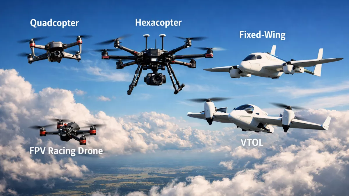
If you are completely new to drones altogether, start with this guide on Types of Drones Explained: Your Complete Beginner’s Guide for 2026 first, then come back here it will make everything below click faster.
Mr. Raj Kumar is a highly experienced Technical Content Engineer with 7 years of dedicated expertise in the intricate field of embedded systems. At Embedded Prep, Raj is at the forefront of creating and curating high-quality technical content designed to educate and empower aspiring and seasoned professionals in the embedded domain.
Throughout his career, Raj has honed a unique skill set that bridges the gap between deep technical understanding and effective communication. His work encompasses a wide range of educational materials, including in-depth tutorials, practical guides, course modules, and insightful articles focused on embedded hardware and software solutions. He possesses a strong grasp of embedded architectures, microcontrollers, real-time operating systems (RTOS), firmware development, and various communication protocols relevant to the embedded industry.
Raj is adept at collaborating closely with subject matter experts, engineers, and instructional designers to ensure the accuracy, completeness, and pedagogical effectiveness of the content. His meticulous attention to detail and commitment to clarity are instrumental in transforming complex embedded concepts into easily digestible and engaging learning experiences. At Embedded Prep, he plays a crucial role in building a robust knowledge base that helps learners master the complexities of embedded technologies.